Bringing the Data Scientist Up to Speed With MerLin

This notebook is tailored for new users with a data science or machine learning background, who want to upgrade their MerLin experience. If you have just started exploring MerLin with the QuantumLayer.simple() method and want a little more expressivity and control on your QuantumLayer, this notebook is made for you ! We will guide you step by step so you can leverage the most ouf of MerLin and unlock both your creativity, and the expressivity of your quantum machine learning models !

MerLins’s QuantumLayer offers much more flexibility that what the simple() method’s is offering. Indeed, it is possible to adapt the interferometer of the layer to our desires easily with the CircuitBuilder.

Run the following imports.

from copy import deepcopy

import matplotlib.pyplot as plt
import numpy as np
import perceval as pcvl
import torch
import torch.nn as nn
import torch.nn.functional as F
from sklearn.datasets import load_digits, load_iris, make_moons
from sklearn.model_selection import train_test_split

import merlin as ML

torch.manual_seed(0)
np.random.seed(0)

simple() recap: classifying iris

The simple() method can be usefull for small classification tasks. Here, we can use it to classify the famous Iris dataset which has 4 features and three flower types.

Let’s first load the data.

iris = load_iris()
X = iris.data.astype("float32")
y = iris.target.astype("int64")

X_train, X_test, y_train, y_test = train_test_split(
    X,
    y,
    test_size=0.25,
    stratify=y,
    random_state=42,
)

X_train = torch.tensor(X_train, dtype=torch.float32)
X_test = torch.tensor(X_test, dtype=torch.float32)
y_train = torch.tensor(y_train, dtype=torch.long)
y_test = torch.tensor(y_test, dtype=torch.long)

mean = X_train.mean(dim=0, keepdim=True)
std = X_train.std(dim=0, keepdim=True).clamp_min(1e-6)
X_train = (X_train - mean) / std
X_test = (X_test - mean) / std

print(f"Train size: {X_train.shape[0]} samples")
print(f"Test size: {X_test.shape[0]} samples")

Train size: 112 samples
Test size: 38 samples

We can then easily create a quantum layer with the simple()method.

quantum_classifier = ML.QuantumLayer.simple(input_size=4, output_size=3)

quantum_classifier

SimpleSequential(
  (quantum_layer): QuantumLayer(
    (_photon_loss_transform): PhotonLossTransform()
    (_detector_transform): DetectorTransform()
    (measurement_mapping): Probabilities()
  )
  (post_processing): ModGrouping()
)

We can use this layer as torch.Module to classify the dataset.

# Simple model training and evaluation process.
def run_experiment(layer: torch.nn.Module, epochs: int = 60, lr: float = 0.05):
    optimizer = torch.optim.Adam(layer.parameters(), lr=lr)
    losses = []
    for _ in range(epochs):
        layer.train()
        optimizer.zero_grad()
        logits = layer(X_train)
        loss = F.cross_entropy(logits, y_train)
        loss.backward()
        optimizer.step()
        losses.append(loss.item())

    layer.eval()
    with torch.no_grad():
        train_preds = layer(X_train).argmax(dim=1)
        test_preds = layer(X_test).argmax(dim=1)
        train_acc = (train_preds == y_train).float().mean().item()
        test_acc = (test_preds == y_test).float().mean().item()
    return losses, train_acc, test_acc


# Running the experiment
test_accs, train_accs = [], []
epochs = [10 * i for i in range(1, 26)]
for epoch in epochs:
    simple_layer = deepcopy(quantum_classifier)
    losses, train_acc, test_acc = run_experiment(simple_layer, epochs=epoch, lr=0.01)
    test_accs.append(test_acc)
    train_accs.append(train_acc)

# Plotting function
plt.plot(epochs, train_accs, label="train")
plt.plot(epochs, test_accs, label="test")
ticks = epochs
indexes_to_pop = []
index = 0
for i in range(len(epochs)):
    if i % 3 > 0:
        ticks.pop(index)
    else:
        index += 1

plt.xticks(ticks=ticks, labels=[str(p) for p in ticks])
plt.xlabel("Epochs")
plt.ylabel("Accuracy")
plt.legend()
plt.show()

What is simple() doing?

The simple method creates an interferometer from the same template every time. Indeed, the circuit that is created has the same number of modes as the number of features+1 and puts a photon every two modes. There is exactly one feature encoded per mode. Here is an example of the circuit for an input size (number of features) of 10.

qlayer = ML.QuantumLayer.simple(input_size=5, output_size=4)

pcvl.pdisplay(qlayer.circuit)

We are limited quickly by computation capabilities as well as photon-number control.

When does simple() becomes not appropriate?

The use of the simple() method is perfect for beginners in photonic QML who just want to explore the quantum capabilities on easy and small datasets. However, we will need to use the full power of the QuamtumLayer to classify more complex and usefull datasets. Indeed, the method only works for datasets that have 19 or less features due to simulation speed reasons. Also, as stated in the Fock State-enhanced Expressivity of Quantum Machine Learning Models paper by Gan et al, the expressivity of a photonic quantum layer is directly related to the number of photons. The simple() method does not allow the user to change in input state of the interferometer.

We will present another easy to use tool to add a QuantumLayer to your torch modules that lets you control the input photons without any feature restrictions.

Transition to merlin.CircuitBuilder

Lets introduce MerLin’s powerful CircuitBuilder. This object can be directly passed to a quantum layer. For a specified number of modes, we can create many interferometer patterns. Lets go deeper to the available patterns.

First, lets create an instance of this object.

circuit_builder = ML.CircuitBuilder(n_modes=2)

circuit_builder

<merlin.builder.circuit_builder.CircuitBuilder at 0x139f24b00>

A) add_rotations()

If we want to add simple rotations on given modes, we can use the add_rotations() method. We can make the parameters trainable and define the starting angle if necessary.

circuit_builder.add_rotations(modes=[0, 1], trainable=True, angle=0.36)

pcvl.pdisplay(circuit_builder.to_pcvl_circuit())

B) add_superposition()

If we want to add a simple interaction on given modes, we can use the add_superposition() method. We can make the parameters trainable, define the starting angles if necessary.

circuit_builder.add_superpositions(modes=[0, 1], theta=0.1, phi=0.15, trainable=True)

pcvl.pdisplay(circuit_builder.to_pcvl_circuit())

C) add_entangling_layer()

If we want a more complex interactions between the modes, we can add an entangling layer. This layer can represent every single interactions between the modes. The parameters can also be trainable. There are two patterns being “mzi” and “bell”. Here we will use the default one being “mzi”.

circuit_builder.add_entangling_layer(modes=[0, 1], trainable=True, model="mzi")

pcvl.pdisplay(circuit_builder.to_pcvl_circuit())

Encoding

Just as simple does, we can add angle encoding to the interferometer. It is how and where the features will be assigned in the boson sampler on a forward pass. It is easy to add with a simple call of the add_angle_encoding() method.

circuit_builder.add_angle_encoding(modes=[0, 1])

pcvl.pdisplay(circuit_builder.to_pcvl_circuit())

Create a QuantumLayer from the CircuitBuilder

Changing the number of photons

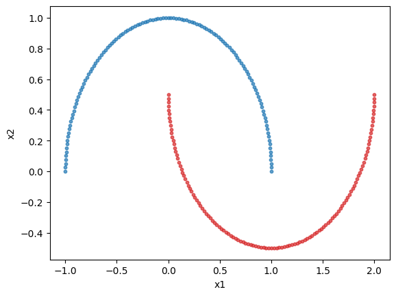
With circuit builder we can now specify the number of photons or the input state of the circuit. Here we will explore the relation between expressivity and the number of photons by classifying the make_moons dataset. It is a dataset with 2 features and 2 classes.

Lets’s first load the dataset

digits = make_moons(n_samples=250)
X = digits[0]
y = digits[1]

X_train, X_test, y_train, y_test = train_test_split(
    X,
    y,
    test_size=0.25,
    stratify=y,
    random_state=42,
)

X_train = torch.tensor(X_train, dtype=torch.float32)
X_test = torch.tensor(X_test, dtype=torch.float32)
y_train = torch.tensor(y_train, dtype=torch.long)
y_test = torch.tensor(y_test, dtype=torch.long)

mean = X_train.mean(dim=0, keepdim=True)
std = X_train.std(dim=0, keepdim=True).clamp_min(1e-6)
X_train = (X_train - mean) / std
X_test = (X_test - mean) / std

print(f"Train size: {X_train.shape[0]} samples")
print(f"Test size: {X_test.shape[0]} samples")

# Plotting the dataset
class_1 = []
class_2 = []

for features, label in zip(X, y, strict=True):
    if label == 0:
        class_1.append(features)
    else:
        class_2.append(features)

class_1 = np.array(class_1)
class_2 = np.array(class_2)

plt.scatter(class_1[:, 0], class_1[:, 1], s=10, color="tab:blue", alpha=0.7)
plt.scatter(class_2[:, 0], class_2[:, 1], s=10, color="tab:red", alpha=0.7)
plt.xlabel("x1")
plt.ylabel("x2")
plt.show()

Train size: 187 samples
Test size: 63 samples

Lets create a 5 mode interferometer with the circuit builder.

moon_circuit = ML.CircuitBuilder(n_modes=5)

moon_circuit.add_entangling_layer()
moon_circuit.add_angle_encoding(modes=[1, 4])
moon_circuit.add_entangling_layer()

pcvl.pdisplay(moon_circuit.to_pcvl_circuit())

Lets run the classification experiment.

# A simple training experiment
def run_experiment(layer: torch.nn.Module, epochs: int = 60, lr: float = 0.05):
    optimizer = torch.optim.Adam(layer.parameters(), lr=lr)
    losses = []
    for _ in range(epochs):
        layer.train()
        optimizer.zero_grad()
        logits = layer(X_train)
        loss = F.cross_entropy(logits, y_train)
        loss.backward()
        optimizer.step()
        losses.append(loss.item())

    layer.eval()
    with torch.no_grad():
        train_preds = layer(X_train).argmax(dim=1)
        test_preds = layer(X_test).argmax(dim=1)
        train_acc = (train_preds == y_train).float().mean().item()
        test_acc = (test_preds == y_test).float().mean().item()
    return losses, train_acc, test_acc

test_accs = [[], [], [], [], []]
epochs = [5 * i for i in range(1, 40)]
for i, num_photons in enumerate([1, 2, 3]):
    for epoch in epochs:
        qcirc = ML.QuantumLayer(builder=deepcopy(moon_circuit), n_photons=num_photons)
        quantum_classifier = nn.Sequential(qcirc, ML.ModGrouping(qcirc.output_size, 2))

        losses, train_acc, test_acc = run_experiment(
            quantum_classifier, epochs=epoch, lr=0.01
        )
        test_accs[i].append(test_acc)


# Plotting function
for i, num_photons in enumerate([1, 2, 3]):
    plt.plot(epochs, test_accs[i], label=f"test (photons={num_photons})")

ticks = epochs.copy()
index = 0
for i in range(len(epochs)):
    if i % 3 > 0:
        ticks.pop(index)
    else:
        index += 1

plt.xticks(ticks=ticks, labels=[str(p) for p in ticks])
plt.xlabel("Epochs")
plt.ylabel("Accuracy")
plt.legend()
plt.show()

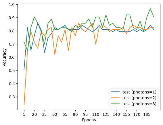
We see that the more the photons, we get better results as the number of epochs increases showing the better expressivity of the model.

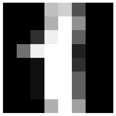
How to encode more features than modes.

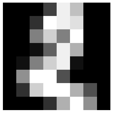
To test the new way of using a QuantumLayer, we will try to classify scikit.learn’s load_digits dataset. It is composed of 8x8 images of hand-written numbers 0 through 9. So, it has 64 features per image, much more than simple() can handle. It is still an easy dataset to classify in theory.

Let’s load the dataset

digits = load_digits()
X = digits.data.astype("float32")
y = digits.target.astype("int64")

X_train, X_test, y_train, y_test = train_test_split(
    X,
    y,
    test_size=0.25,
    stratify=y,
    random_state=42,
)

X_train = torch.tensor(X_train, dtype=torch.float32)
X_test = torch.tensor(X_test, dtype=torch.float32)
y_train = torch.tensor(y_train, dtype=torch.long)
y_test = torch.tensor(y_test, dtype=torch.long)

mean = X_train.mean(dim=0, keepdim=True)
std = X_train.std(dim=0, keepdim=True).clamp_min(1e-6)
X_train = (X_train - mean) / std
X_test = (X_test - mean) / std

print(f"Train size: {X_train.shape[0]} samples")
print(f"Test size: {X_test.shape[0]} samples")

# Plot the first 5 digits
for i in range(5):
    plt.imshow(digits.images[i], cmap="gray")
    plt.axis("off")
    plt.show()

Train size: 1347 samples
Test size: 450 samples

Let’s create a circuit with 8 modes and 8 angle encoding layers.

circuit = ML.CircuitBuilder(n_modes=8)

circuit.add_entangling_layer()
for _ in range(8):
    circuit.add_angle_encoding()
    circuit.add_entangling_layer()

pcvl.pdisplay(circuit.to_pcvl_circuit())

Lets run the classification experiment

# A simple training experiment
def run_experiment(layer: torch.nn.Module, epochs: int = 60, lr: float = 0.05):
    optimizer = torch.optim.Adam(layer.parameters(), lr=lr)
    losses = []
    test_accuracies = []
    train_accuracies = []
    for i in range(epochs):
        layer.train()
        optimizer.zero_grad()
        logits = layer(X_train)
        loss = F.cross_entropy(logits, y_train)
        loss.backward()
        optimizer.step()
        losses.append(loss.item())

        layer.eval()
        with torch.no_grad():
            train_preds = layer(X_train).argmax(dim=1)
            test_preds = layer(X_test).argmax(dim=1)
            train_acc = (train_preds == y_train).float().mean().item()
            test_acc = (test_preds == y_test).float().mean().item()
            test_accuracies.append(test_acc)
            train_accuracies.append(train_acc)
        layer.train()
        if (i+1)%25==0:
            print(
                f"Epoch {i + 1} had a loss of {losses[-1]}, a training accuracy of {train_acc} and a testing accuracy of {test_acc}"
            )

    layer.eval()
    return losses, train_accuracies, test_accuracies

To give the right output size, we will use a ML.ModGroupingstrategy to make sure was have an output dimension of 10. It combines the outputs of the quantum circuit in a dimension 10 vector (one dimension per class).

# Running the experiment
epochs = 500

qcirc = ML.QuantumLayer(builder=deepcopy(circuit), n_photons=1)
quantum_classifier = nn.Sequential(qcirc, ML.ModGrouping(qcirc.output_size, 10))

losses, train_acc, test_acc = run_experiment(quantum_classifier, epochs=epochs, lr=0.01)

# Plotting function
plt.plot(list(range(1, epochs + 1)), train_acc, label="train")
plt.plot(list(range(1, epochs + 1)), test_acc, label="test")
ticks = list(range(1, epochs + 1))
indexes_to_pop = []
index = 0
for i in range(1, epochs + 1):
    if i % 100 > 0:
        ticks.pop(index)
    else:
        index += 1

plt.xticks(ticks=ticks, labels=[str(p) for p in ticks])
plt.xlabel("Epochs")
plt.ylabel("Accuracy")
plt.legend()
plt.show()

Epoch 25 had a loss of 2.174989938735962, a training accuracy of 0.41128432750701904 and a testing accuracy of 0.3733333349227905
Epoch 50 had a loss of 2.1213064193725586, a training accuracy of 0.5040831565856934 and a testing accuracy of 0.48444443941116333
Epoch 75 had a loss of 2.065514326095581, a training accuracy of 0.5946547985076904 and a testing accuracy of 0.5933333039283752
Epoch 100 had a loss of 2.0221264362335205, a training accuracy of 0.6481069326400757 and a testing accuracy of 0.653333306312561
Epoch 125 had a loss of 1.9971283674240112, a training accuracy of 0.6748329401016235 and a testing accuracy of 0.6733333468437195
Epoch 150 had a loss of 1.980004906654358, a training accuracy of 0.6889383792877197 and a testing accuracy of 0.6822222471237183
Epoch 175 had a loss of 1.9685148000717163, a training accuracy of 0.6948775053024292 and a testing accuracy of 0.6800000071525574
Epoch 200 had a loss of 1.9598309993743896, a training accuracy of 0.7030438184738159 and a testing accuracy of 0.6933333277702332
Epoch 225 had a loss of 1.9529314041137695, a training accuracy of 0.7045285701751709 and a testing accuracy of 0.695555567741394
Epoch 250 had a loss of 1.9475393295288086, a training accuracy of 0.7060133814811707 and a testing accuracy of 0.695555567741394
Epoch 275 had a loss of 1.9434336423873901, a training accuracy of 0.7067557573318481 and a testing accuracy of 0.699999988079071
Epoch 300 had a loss of 1.9402966499328613, a training accuracy of 0.7067557573318481 and a testing accuracy of 0.6933333277702332
Epoch 325 had a loss of 1.9376776218414307, a training accuracy of 0.7074981331825256 and a testing accuracy of 0.6822222471237183
Epoch 350 had a loss of 1.9351595640182495, a training accuracy of 0.7067557573318481 and a testing accuracy of 0.6800000071525574
Epoch 375 had a loss of 1.9324162006378174, a training accuracy of 0.7067557573318481 and a testing accuracy of 0.6755555272102356
Epoch 400 had a loss of 1.9293900728225708, a training accuracy of 0.7089829444885254 and a testing accuracy of 0.6733333468437195
Epoch 425 had a loss of 1.926409125328064, a training accuracy of 0.7082405090332031 and a testing accuracy of 0.6822222471237183
Epoch 450 had a loss of 1.9238649606704712, a training accuracy of 0.7134372591972351 and a testing accuracy of 0.6911110877990723
Epoch 475 had a loss of 1.9218140840530396, a training accuracy of 0.7112100720405579 and a testing accuracy of 0.6911110877990723
Epoch 500 had a loss of 1.9201419353485107, a training accuracy of 0.7097253203392029 and a testing accuracy of 0.6933333277702332

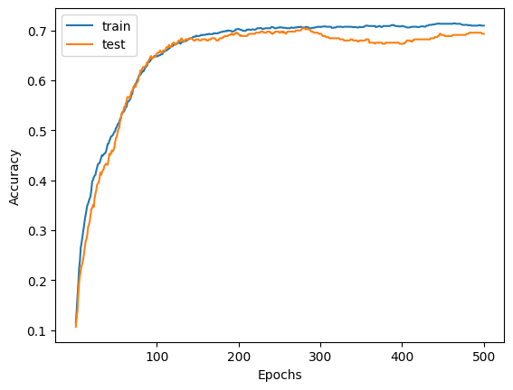
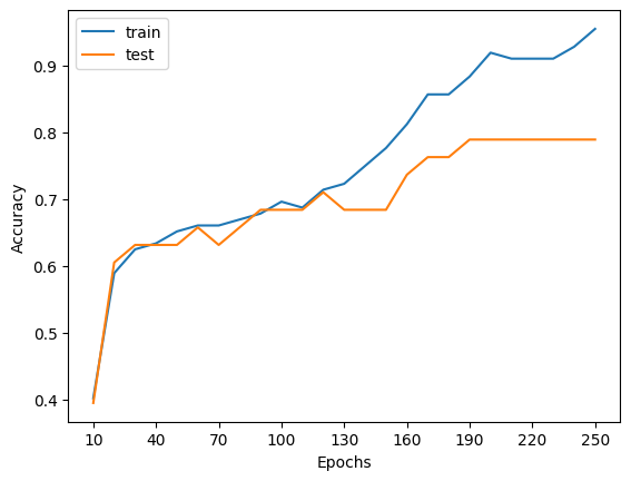
We observe that with 8 times less modes that simple() would need, we are still able to classify the dataset.

Here you go! You are now ready to take advantage of the full power of MerLin’s QuantumLayer! The next step in your journey would be to investigate the different data encoding in the quantum circuits which can be found on the angle amplitude encoding page.