Quantum-Classical Hybrid Neural Network Comparison
This notebook compares different neural network architectures including:
Classical Multi-Layer Perceptrons (MLP)
Quantum circuits with LINEAR output mapping
Quantum circuits with various GROUPING strategies
1. Import Required Libraries
First, we’ll import all necessary libraries for our experiment:
PyTorch: For neural network implementation and training
Perceval: For quantum circuit simulation
Matplotlib/Seaborn: For visualization
Custom modules: For quantum layers and MLP models
[ ]:
from collections import defaultdict

import matplotlib.pyplot as plt
import perceval as pcvl
import seaborn as sns
import torch
import torch.nn as nn
from sklearn.metrics import accuracy_score, classification_report, confusion_matrix
from tqdm import tqdm

%matplotlib inline

from merlin import (
    ComputationSpace,
    LexGrouping,
    MeasurementStrategy,
    ModGrouping,
    QuantumLayer,
)
from merlin.datasets import iris
p ## 2. Load and Prepare the Iris Dataset
We’ll use the classic Iris dataset for multi-class classification. This dataset is ideal for comparing different architectures as it provides a simple but non-trivial classification task.
The dataset contains:
4 features: sepal length, sepal width, petal length, petal width
3 classes: Setosa, Versicolor, Virginica
150 samples total (split into train/test sets)
[3]:
train_features, train_labels, train_metadata = iris.get_data_train()
test_features, test_labels, test_metadata = iris.get_data_test()

# Convert data to PyTorch tensors
X_train = torch.FloatTensor(train_features)
y_train = torch.LongTensor(train_labels)
X_test = torch.FloatTensor(test_features)
y_test = torch.LongTensor(test_labels)

print(f"Training samples: {X_train.shape[0]}")
print(f"Test samples: {X_test.shape[0]}")
print(f"Features: {X_train.shape[1]}")
print(f"Classes: {len(torch.unique(y_train))}")
Training samples: 120
Test samples: 30
Features: 4
Classes: 3
## 3. Define Model Variants
We’ll test several model architectures to compare classical and quantum approaches:
Classical Models:
MLP: Multi-layer perceptron with 8 hidden units, ReLU activation, and 0.1 dropout
Quantum Models:
LINEAR-7modes-nobunching: Uses linear output mapping with 7 quantum modes and no-bunching constraintLEXGROUPING-7modes: Uses lexicographic grouping strategy for output mappingMODGROUPING-7modes: Uses modular grouping strategy for output mapping
Each model type has a distinct color and line style for visualization.
[4]:
from dataclasses import dataclass
from typing import Literal

import torch


@dataclass
class MLPConfig:
    """Configuration for Multi-Layer Perceptron"""

    hidden_sizes: list[int] = None
    dropout: float = 0.0
    activation: Literal[
        "relu", "tanh", "sigmoid", "leaky_relu", "elu", "gelu", "selu"
    ] = "relu"
    normalization: Literal["batch", "layer"] | None = None


class MLP(nn.Module):
    """
    An enhanced Multi-Layer Perceptron (MLP) implementation with customizable options.

    Features:
    - Multiple activation functions
    - Batch/Layer normalization options
    - Customizable weight initialization

    Args:
        input_size (int): Dimension of the input features
        output_size (int): Dimension of the output
        config (MLPConfig): Configuration for the network architecture
    """

    # Class-level mapping of available activation functions
    ACTIVATIONS = {
        "relu": nn.ReLU(),
        "tanh": nn.Tanh(),
        "sigmoid": nn.Sigmoid(),
        "leaky_relu": nn.LeakyReLU(),
        "elu": nn.ELU(),
        "gelu": nn.GELU(),
        "selu": nn.SELU(),
    }

    def __init__(self, input_size: int, output_size: int, config: MLPConfig):
        super().__init__()
        last_layer_size = input_size
        layers = []

        self.config = config

        # Validate activation function
        if config.activation not in self.ACTIVATIONS:
            raise ValueError(f"Unsupported activation function: {config.activation}")

        # Build network architecture
        for layer_size in config.hidden_sizes:
            # Add linear layer
            layers.append(nn.Linear(last_layer_size, layer_size))

            # Add normalization if specified
            if config.normalization == "batch":
                layers.append(nn.BatchNorm1d(layer_size))
            elif config.normalization == "layer":
                layers.append(nn.LayerNorm(layer_size))

            # Add activation function
            layers.append(self.ACTIVATIONS[config.activation])

            # Add dropout if specified
            if config.dropout > 0:
                layers.append(nn.Dropout(config.dropout))

            last_layer_size = layer_size

        # Add final output layer
        layers.append(nn.Linear(last_layer_size, output_size))

        # Create sequential model from layers
        self.network = nn.Sequential(*layers)

    def initialize_weights(self, method="xavier"):
        """
        Initialize network weights using the specified method.

        Args:
            method (str): Initialization method ('xavier' or 'kaiming') (default: 'xavier')
        """

        for layer in self.network:
            if isinstance(layer, nn.Linear):
                if method == "xavier":
                    nn.init.xavier_uniform_(layer.weight)
                    nn.init.zeros_(layer.bias)
                elif method == "kaiming":
                    nn.init.kaiming_normal_(layer.weight, nonlinearity="relu")
                    nn.init.zeros_(layer.bias)
                else:
                    raise ValueError(f"Unsupported initialization method: {method}")

    def forward(self, x):
        """
        Forward pass of the network.

        Args:
            x (torch.Tensor): Input tensor with shape (batch_size, input_size)

        Returns:
            torch.Tensor: Output tensor with shape (batch_size, output_size)
        """
        return self.network(x)
[5]:
def get_model_variants():
    """Define different variants for each model type"""
    # Define consistent colors for each model type
    MODEL_COLORS = {
        "MLP": "#1f77b4",  # Blue
        "LINEAR": "#2ca02c",  # Green
        "GROUPING": "#ff7f0e",  # Orange
    }

    # Define line styles for variants
    LINE_STYLES = ["--", "-", ":", "-."]

    variants = {
        "MLP": [
            {
                "name": "MLP",
                "config": MLPConfig(hidden_sizes=[8], dropout=0.1, activation="relu"),
                "color": MODEL_COLORS["MLP"],
                "linestyle": LINE_STYLES[0],
            }
        ],
        "LINEAR": [
            {
                "name": "LINEAR-7modes-nobunching",
                "config": {
                    "m": 7,
                    "post_processing": "linear",
                    "no_bunching": True,
                },
                "color": MODEL_COLORS["LINEAR"],
                "linestyle": LINE_STYLES[1],
            }
        ],
        "GROUPING": [
            {
                "name": "LEXGROUPING-7modes",
                "config": {
                    "m": 6,
                    "post_processing": "lex",
                },
                "color": MODEL_COLORS["GROUPING"],
                "linestyle": LINE_STYLES[2],
            },
            {
                "name": "MODGROUPING-7modes",
                "config": {
                    "m": 6,
                    "post_processing": "mod",
                },
                "color": MODEL_COLORS["GROUPING"],
                "linestyle": LINE_STYLES[1],
            },
        ],
    }
    return variants
## 4. Quantum Circuit Architecture
The quantum circuit is composed of three main sections:
Left interferometer (WL): Performs initial quantum state transformation using beam splitters and phase shifters
Variable phase shifters: Encodes the 4 input features into quantum phases
Right interferometer (WR): Performs final quantum state transformation
The interferometers use a rectangular arrangement of optical elements, where each layer consists of beam splitters (BS) and programmable phase shifters (PS). The phase shifters contain trainable parameters that are optimized during training.
[6]:
def create_quantum_circuit(m):
    """Create quantum circuit with specified number of modes

    Parameters:
    -----------
    m : int
        Number of quantum modes in the circuit

    Returns:
    --------
    pcvl.Circuit
        Complete quantum circuit with trainable parameters
    """
    # Left interferometer with trainable parameters
    wl = pcvl.GenericInterferometer(
        m,
        lambda i: (
            pcvl.BS()
            // pcvl.PS(pcvl.P(f"theta_li{i}"))
            // pcvl.BS()
            // pcvl.PS(pcvl.P(f"theta_lo{i}"))
        ),
        shape=pcvl.InterferometerShape.RECTANGLE,
    )

    # Variable phase shifters for input encoding
    c_var = pcvl.Circuit(m)
    for i in range(4):  # 4 input features
        px = pcvl.P(f"px{i + 1}")
        c_var.add(i + (m - 4) // 2, pcvl.PS(px))

    # Right interferometer with trainable parameters
    wr = pcvl.GenericInterferometer(
        m,
        lambda i: (
            pcvl.BS()
            // pcvl.PS(pcvl.P(f"theta_ri{i}"))
            // pcvl.BS()
            // pcvl.PS(pcvl.P(f"theta_ro{i}"))
        ),
        shape=pcvl.InterferometerShape.RECTANGLE,
    )

    # Combine all components
    c = pcvl.Circuit(m)
    c.add(0, wl, merge=True)
    c.add(0, c_var, merge=True)
    c.add(0, wr, merge=True)

    return c
## 5. Model Factory Functions
These utility functions handle model creation and parameter counting. The create_model function serves as a factory that instantiates either classical MLP models or quantum models based on the specified configuration.
[7]:
def create_model(model_type, variant):
    """Create model instance based on type and variant

    Parameters:
    -----------
    model_type : str
        Type of model ('MLP' or quantum model types)
    variant : dict
        Configuration dictionary for the model variant

    Returns:
    --------
    nn.Module
        PyTorch model instance
    """
    if model_type == "MLP":
        return MLP(input_size=4, output_size=3, config=variant["config"])
    else:
        m = variant["config"]["m"]
        no_bunching = variant["config"].get("no_bunching", False)
        post_processing = variant["config"].get("post_processing")
        c = create_quantum_circuit(m)
        quantum_layer = QuantumLayer(
            input_size=4,
            circuit=c,
            trainable_parameters=["theta"],
            input_parameters=["px"],
            input_state=[1, 0] * (m // 2) + [0] * (m % 2),
            measurement_strategy=MeasurementStrategy.probs(
                computation_space=ComputationSpace.UNBUNCHED
                if no_bunching
                else ComputationSpace.FOCK
            ),
        )

        if post_processing == "linear":
            head = nn.Linear(quantum_layer.output_size, 3)
            return nn.Sequential(quantum_layer, head)
        if post_processing == "lex":
            return nn.Sequential(
                quantum_layer,
                LexGrouping(quantum_layer.output_size, 3),
            )
        if post_processing == "mod":
            return nn.Sequential(
                quantum_layer,
                ModGrouping(quantum_layer.output_size, 3),
            )
        return quantum_layer


def count_parameters(model):
    """Count trainable parameters in a PyTorch model"""
    return sum(p.numel() for p in model.parameters() if p.requires_grad)
## 6. Training Function
The training function implements a standard supervised learning loop with the following characteristics:
Optimizer: Adam with learning rate 0.02
Loss function: Cross-entropy for multi-class classification
Batch size: 32 samples
Epochs: 50 (default)
The function tracks training loss, training accuracy, and test accuracy at each epoch. After training completes, it generates a detailed classification report.
[8]:
def train_model(
    model,
    X_train,
    y_train,
    X_test,
    y_test,
    model_name,
    n_epochs=50,
    batch_size=32,
    lr=0.02,
):
    """Train a model and track metrics

    Parameters:
    -----------
    model : nn.Module
        Model to train
    X_train, y_train : torch.Tensor
        Training data and labels
    X_test, y_test : torch.Tensor
        Test data and labels
    model_name : str
        Name for progress bar display
    n_epochs : int
        Number of training epochs
    batch_size : int
        Batch size for mini-batch training
    lr : float
        Learning rate

    Returns:
    --------
    dict
        Training results including losses, accuracies, and final report
    """
    optimizer = torch.optim.Adam(model.parameters(), lr=lr)
    criterion = nn.CrossEntropyLoss()

    losses = []
    train_accuracies = []
    test_accuracies = []

    model.train()

    pbar = tqdm(range(n_epochs), leave=False, desc=f"Training {model_name}")
    for _epoch in pbar:
        # Shuffle training data
        permutation = torch.randperm(X_train.size()[0])
        total_loss = 0

        # Mini-batch training
        for i in range(0, X_train.size()[0], batch_size):
            indices = permutation[i : i + batch_size]
            batch_x, batch_y = X_train[indices], y_train[indices]

            outputs = model(batch_x)
            loss = criterion(outputs, batch_y)

            optimizer.zero_grad()
            loss.backward()
            optimizer.step()

            total_loss += loss.item()

        avg_loss = total_loss / (X_train.size()[0] // batch_size)
        losses.append(avg_loss)
        pbar.set_description(f"Training {model_name} - Loss: {avg_loss:.4f}")

        # Evaluation
        model.eval()
        with torch.no_grad():
            # Training accuracy
            train_outputs = model(X_train)
            train_preds = torch.argmax(train_outputs, dim=1).numpy()
            train_acc = accuracy_score(y_train.numpy(), train_preds)
            train_accuracies.append(train_acc)

            # Test accuracy
            test_outputs = model(X_test)
            test_preds = torch.argmax(test_outputs, dim=1).numpy()
            test_acc = accuracy_score(y_test.numpy(), test_preds)
            test_accuracies.append(test_acc)

        model.train()

    # Generate final classification report
    model.eval()
    with torch.no_grad():
        final_test_outputs = model(X_test)
        final_test_preds = torch.argmax(final_test_outputs, dim=1).numpy()
        final_report = classification_report(y_test.numpy(), final_test_preds)

    return {
        "losses": losses,
        "train_accuracies": train_accuracies,
        "test_accuracies": test_accuracies,
        "final_test_acc": test_accuracies[-1],
        "classification_report": final_report,
    }
## 7. Multi-Run Training Function
To ensure robust and statistically meaningful results, we train each model variant multiple times with different random initializations. This approach helps us:
Understand the variance in model performance
Identify which architectures are more stable
Avoid drawing conclusions from lucky/unlucky single runs
Calculate confidence intervals for performance metrics
The function tracks both individual run results and aggregate statistics across all runs.
[9]:
def train_all_variants(X_train, y_train, X_test, y_test, num_runs=5):
    """Train all model variants multiple times and return results

    Parameters:
    -----------
    X_train, y_train : torch.Tensor
        Training data and labels
    X_test, y_test : torch.Tensor
        Test data and labels
    num_runs : int
        Number of independent training runs per variant

    Returns:
    --------
    tuple
        (all_results, best_models) - Complete results and best performing models
    """
    variants = get_model_variants()
    all_results = defaultdict(dict)
    best_models = {}

    for model_type, model_variants in variants.items():
        print(f"\n\nTraining {model_type} variants:")
        best_acc = 0

        for variant in model_variants:
            print(
                f"\nTraining {variant['name']}... ({count_parameters(create_model(model_type, variant))} parameters)"
            )

            # Store results from multiple runs
            variant_runs = []

            for run in range(num_runs):
                model = create_model(model_type, variant)
                print(f"  Run {run + 1}/{num_runs}...")

                results = train_model(
                    model,
                    X_train,
                    y_train,
                    X_test,
                    y_test,
                    f"{variant['name']}-run{run + 1}",
                )
                results["model"] = model
                results["color"] = variant["color"]
                results["linestyle"] = variant["linestyle"]
                variant_runs.append(results)

                # Track best model for each type
                if results["final_test_acc"] > best_acc:
                    best_acc = results["final_test_acc"]
                    best_models[model_type] = {
                        "name": variant["name"],
                        "model": model,
                        "results": results,
                    }

            # Store all runs for this variant
            all_results[model_type][variant["name"]] = {
                "runs": variant_runs,
                "color": variant["color"],
                "linestyle": variant["linestyle"],
                "avg_final_test_acc": sum(run["final_test_acc"] for run in variant_runs)
                / num_runs,
            }

    return all_results, best_models
## 8. Visualization Functions
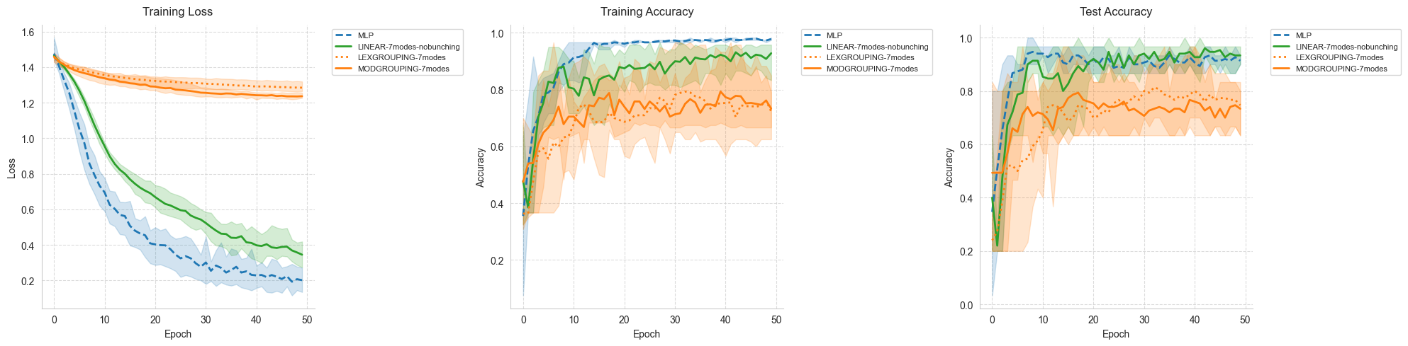
### Training Curves Visualization
This function creates a comprehensive view of the training process by plotting three key metrics:
Training Loss: Shows how well the model fits the training data
Training Accuracy: Indicates the model’s performance on training samples
Test Accuracy: Reveals the model’s generalization capability
For each model variant, we display:
Solid line: Mean performance across all runs
Shaded area: Performance envelope (min to max values)
This visualization helps identify overfitting, convergence speed, and stability.
[10]:
def plot_training_curves(all_results):
    """Plot training curves for all model variants with average and envelope

    Shows three subplots:
    1. Training loss over epochs
    2. Training accuracy over epochs
    3. Test accuracy over epochs

    Each line represents the mean across runs, with shaded areas showing min/max envelope.
    """
    fig, (ax1, ax2, ax3) = plt.subplots(1, 3, figsize=(20, 5))

    # Plot each metric
    for _model_type, variants in all_results.items():
        for variant_name, variant_data in variants.items():
            color = variant_data["color"]
            linestyle = variant_data["linestyle"]
            label = f"{variant_name}"

            # Get data from all runs
            losses_runs = [run["losses"] for run in variant_data["runs"]]
            train_acc_runs = [run["train_accuracies"] for run in variant_data["runs"]]
            test_acc_runs = [run["test_accuracies"] for run in variant_data["runs"]]

            # Calculate mean values across all runs
            epochs = len(losses_runs[0])
            mean_losses = [
                sum(run[i] for run in losses_runs) / len(losses_runs)
                for i in range(epochs)
            ]
            mean_train_acc = [
                sum(run[i] for run in train_acc_runs) / len(train_acc_runs)
                for i in range(epochs)
            ]
            mean_test_acc = [
                sum(run[i] for run in test_acc_runs) / len(test_acc_runs)
                for i in range(epochs)
            ]

            # Calculate min and max values for the envelope
            min_losses = [min(run[i] for run in losses_runs) for i in range(epochs)]
            max_losses = [max(run[i] for run in losses_runs) for i in range(epochs)]

            min_train_acc = [
                min(run[i] for run in train_acc_runs) for i in range(epochs)
            ]
            max_train_acc = [
                max(run[i] for run in train_acc_runs) for i in range(epochs)
            ]

            min_test_acc = [min(run[i] for run in test_acc_runs) for i in range(epochs)]
            max_test_acc = [max(run[i] for run in test_acc_runs) for i in range(epochs)]

            # Plot mean lines
            ax1.plot(
                mean_losses, label=label, color=color, linestyle=linestyle, linewidth=2
            )
            ax2.plot(
                mean_train_acc,
                label=label,
                color=color,
                linestyle=linestyle,
                linewidth=2,
            )
            ax3.plot(
                mean_test_acc,
                label=label,
                color=color,
                linestyle=linestyle,
                linewidth=2,
            )

            # Plot envelopes (filled area between min and max)
            epochs_range = range(epochs)
            ax1.fill_between(
                epochs_range, min_losses, max_losses, color=color, alpha=0.2
            )
            ax2.fill_between(
                epochs_range, min_train_acc, max_train_acc, color=color, alpha=0.2
            )
            ax3.fill_between(
                epochs_range, min_test_acc, max_test_acc, color=color, alpha=0.2
            )

    # Customize plots
    for ax, title in zip(
        [ax1, ax2, ax3],
        ["Training Loss", "Training Accuracy", "Test Accuracy"],
        strict=False,
    ):
        ax.set_title(title, fontsize=12, pad=10)
        ax.set_xlabel("Epoch", fontsize=10)
        ax.set_ylabel(title.split()[-1], fontsize=10)
        ax.legend(fontsize=8, bbox_to_anchor=(1.05, 1), loc="upper left")
        ax.grid(True, linestyle="--", alpha=0.7)
        ax.spines["top"].set_visible(False)
        ax.spines["right"].set_visible(False)

    plt.tight_layout()
    plt.show()
### Confusion Matrix Visualization
Confusion matrices provide detailed insights into classification performance by showing:
Which classes are correctly classified (diagonal elements)
Which classes are confused with each other (off-diagonal elements)
Overall performance patterns for each model architecture
We display the confusion matrix for the best-performing model of each type.
[11]:
def plot_best_confusion_matrices(best_models, X_test, y_test):
    """Plot confusion matrices for the best model of each type"""
    fig, axes = plt.subplots(1, 3, figsize=(20, 5))
    class_names = ["setosa", "versicolor", "virginica"]

    for idx, (model_type, best) in enumerate(best_models.items()):
        model = best["model"]
        model.eval()
        with torch.no_grad():
            outputs = model(X_test)
            predictions = torch.argmax(outputs, dim=1).numpy()

        cm = confusion_matrix(y_test.numpy(), predictions)
        sns.heatmap(
            cm,
            annot=True,
            fmt="d",
            cmap="Blues",
            xticklabels=class_names,
            yticklabels=class_names,
            ax=axes[idx],
        )
        axes[idx].set_title(f"Best {model_type}\n({best['name']})")
        axes[idx].set_xlabel("Predicted")
        axes[idx].set_ylabel("True")
        plt.setp(axes[idx].get_xticklabels(), rotation=45)
        plt.setp(axes[idx].get_yticklabels(), rotation=45)

    plt.tight_layout()
    plt.show()
## 9. Results Summary Function
This function provides a comprehensive statistical analysis of the experimental results, including:
Parameter efficiency: Number of trainable parameters for each model
Performance statistics: Mean accuracy, standard deviation, min/max values
Detailed classification reports: Precision, recall, and F1-score for each class
These metrics help in making informed decisions about model selection based on the specific requirements of your application.
[12]:
def print_comparison_results(all_results, best_models):
    """Print detailed comparison of all models and variants with multi-run statistics"""
    print("\n----- Model Comparison Results -----")

    # Print results for all variants
    print("\nAll Model Variants Results (averaged over multiple runs):")
    for model_type, variants in all_results.items():
        print(f"\n{model_type} Variants:")
        for variant_name, variant_data in variants.items():
            print(f"\n{variant_name}:")
            print(f"Parameters: {count_parameters(variant_data['runs'][0]['model'])}")

            # Calculate statistics across runs
            final_accs = [run["final_test_acc"] for run in variant_data["runs"]]
            avg_acc = sum(final_accs) / len(final_accs)
            min_acc = min(final_accs)
            max_acc = max(final_accs)
            std_acc = (
                sum((acc - avg_acc) ** 2 for acc in final_accs) / len(final_accs)
            ) ** 0.5

            print(
                f"Final Test Accuracy: {avg_acc:.4f} ± {std_acc:.4f} (min: {min_acc:.4f}, max: {max_acc:.4f})"
            )

    # Print best model results
    print("\nBest Models:")
    for model_type, best in best_models.items():
        print(f"\nBest {model_type} Model: {best['name']}")
        print(f"Final Test Accuracy: {best['results']['final_test_acc']:.4f}")
        print(f"Classification Report:\n{best['results']['classification_report']}")
## 10. Run the Complete Experiment
Now we’ll execute the full experimental pipeline. The experiment consists of:
Multiple training runs: Each model variant is trained 5 times with different random seeds
Performance tracking: All metrics are recorded for statistical analysis
Visualization: Training curves and confusion matrices are generated
Statistical summary: Detailed performance statistics are computed
This comprehensive approach ensures reliable and reproducible results.
[13]:
# Set number of independent runs per model variant
num_runs = 5

# Train all variants
print("Starting training process...")
all_results, best_models = train_all_variants(
    X_train, y_train, X_test, y_test, num_runs=num_runs
)
Starting training process...


Training MLP variants:

Training MLP... (67 parameters)
  Run 1/5...
Run 2/5...
Run 3/5...
Run 4/5...
Run 5/5...
Training LINEAR variants:

Training LINEAR-7modes-nobunching... (192 parameters)
  Run 1/5...
Run 2/5...
Run 3/5...
Run 4/5...
Run 5/5...
Training GROUPING variants:

Training LEXGROUPING-7modes... (60 parameters)
  Run 1/5...
/Users/lfvigneux/miniconda3/envs/MerLin_dev/lib/python3.12/site-packages/sklearn/metrics/_classification.py:1833: UndefinedMetricWarning: Precision is ill-defined and being set to 0.0 in labels with no predicted samples. Use `zero_division` parameter to control this behavior.
  _warn_prf(average, modifier, f"{metric.capitalize()} is", result.shape[0])
Run 2/5...
Run 3/5...
Run 4/5...
Run 5/5...
Training MODGROUPING-7modes... (60 parameters)
  Run 1/5...
/Users/lfvigneux/miniconda3/envs/MerLin_dev/lib/python3.12/site-packages/sklearn/metrics/_classification.py:1833: UndefinedMetricWarning: Precision is ill-defined and being set to 0.0 in labels with no predicted samples. Use `zero_division` parameter to control this behavior.
  _warn_prf(average, modifier, f"{metric.capitalize()} is", result.shape[0])
/Users/lfvigneux/miniconda3/envs/MerLin_dev/lib/python3.12/site-packages/sklearn/metrics/_classification.py:1833: UndefinedMetricWarning: Precision is ill-defined and being set to 0.0 in labels with no predicted samples. Use `zero_division` parameter to control this behavior.
  _warn_prf(average, modifier, f"{metric.capitalize()} is", result.shape[0])
/Users/lfvigneux/miniconda3/envs/MerLin_dev/lib/python3.12/site-packages/sklearn/metrics/_classification.py:1833: UndefinedMetricWarning: Precision is ill-defined and being set to 0.0 in labels with no predicted samples. Use `zero_division` parameter to control this behavior.
  _warn_prf(average, modifier, f"{metric.capitalize()} is", result.shape[0])
Run 2/5...
/Users/lfvigneux/miniconda3/envs/MerLin_dev/lib/python3.12/site-packages/sklearn/metrics/_classification.py:1833: UndefinedMetricWarning: Precision is ill-defined and being set to 0.0 in labels with no predicted samples. Use `zero_division` parameter to control this behavior.
  _warn_prf(average, modifier, f"{metric.capitalize()} is", result.shape[0])
Run 3/5...
Run 4/5...
/Users/lfvigneux/miniconda3/envs/MerLin_dev/lib/python3.12/site-packages/sklearn/metrics/_classification.py:1833: UndefinedMetricWarning: Precision is ill-defined and being set to 0.0 in labels with no predicted samples. Use `zero_division` parameter to control this behavior.
  _warn_prf(average, modifier, f"{metric.capitalize()} is", result.shape[0])
Run 5/5...
/Users/lfvigneux/miniconda3/envs/MerLin_dev/lib/python3.12/site-packages/sklearn/metrics/_classification.py:1833: UndefinedMetricWarning: Precision is ill-defined and being set to 0.0 in labels with no predicted samples. Use `zero_division` parameter to control this behavior.
  _warn_prf(average, modifier, f"{metric.capitalize()} is", result.shape[0])
### Visualize Training Progress
The following plots show how each model’s performance evolves during training. Pay attention to:
Convergence speed: How quickly each model reaches its best performance
Stability: Width of the shaded area indicates variance across runs
Final performance: Where each model plateaus
[14]:
plot_training_curves(all_results)
### Confusion Matrices for Best Models
These confusion matrices reveal the classification patterns of the best-performing model from each architecture type. Look for:
Perfect classification: Bright blue diagonal with zeros elsewhere
Common confusions: Off-diagonal elements show which classes are hard to distinguish
[15]:
print_comparison_results(all_results, best_models)
----- Model Comparison Results -----

All Model Variants Results (averaged over multiple runs):

MLP Variants:

MLP:
Parameters: 67
Final Test Accuracy: 0.9267 ± 0.0249 (min: 0.9000, max: 0.9667)

LINEAR Variants:

LINEAR-7modes-nobunching:
Parameters: 192
Final Test Accuracy: 0.9200 ± 0.0452 (min: 0.8667, max: 0.9667)

GROUPING Variants:

LEXGROUPING-7modes:
Parameters: 60
Final Test Accuracy: 0.8333 ± 0.1116 (min: 0.6333, max: 0.9667)

MODGROUPING-7modes:
Parameters: 60
Final Test Accuracy: 0.6733 ± 0.0800 (min: 0.6333, max: 0.8333)

Best Models:

Best MLP Model: MLP
Final Test Accuracy: 0.9667
Classification Report:
              precision    recall  f1-score   support

           0       1.00      1.00      1.00        13
           1       0.86      1.00      0.92         6
           2       1.00      0.91      0.95        11

    accuracy                           0.97        30
   macro avg       0.95      0.97      0.96        30
weighted avg       0.97      0.97      0.97        30


Best LINEAR Model: LINEAR-7modes-nobunching
Final Test Accuracy: 0.9667
Classification Report:
              precision    recall  f1-score   support

           0       1.00      1.00      1.00        13
           1       0.86      1.00      0.92         6
           2       1.00      0.91      0.95        11

    accuracy                           0.97        30
   macro avg       0.95      0.97      0.96        30
weighted avg       0.97      0.97      0.97        30


Best GROUPING Model: LEXGROUPING-7modes
Final Test Accuracy: 0.9667
Classification Report:
              precision    recall  f1-score   support

           0       1.00      1.00      1.00        13
           1       0.86      1.00      0.92         6
           2       1.00      0.91      0.95        11

    accuracy                           0.97        30
   macro avg       0.95      0.97      0.96        30
weighted avg       0.97      0.97      0.97        30
## 11. Key Findings and Conclusions
Based on the experimental results, we can draw several important conclusions:
Model Complexity vs Performance:
Compare the number of parameters required by each architecture
Assess whether quantum models achieve similar performance with fewer parameters
Training Stability:
The variance across multiple runs indicates how sensitive each model is to initialization
Lower variance suggests more reliable training
Generalization Capability:
The gap between training and test accuracy reveals overfitting tendencies
Smaller gaps indicate better generalization
Classification Patterns:
Confusion matrices show which flower species are most difficult to distinguish
This can guide feature engineering or model selection
Practical Considerations:
For deployment, consider:
Classical MLPs: Well-understood, fast inference, established deployment pipelines
Quantum models: Potentially more parameter-efficient, may offer advantages on quantum hardware
Future Research Directions:
Scaling to larger datasets: Test on more complex classification tasks
Noise modeling: Investigate performance under realistic quantum noise conditions
Hybrid architectures: Combine classical and quantum layers
Hardware implementation: Evaluate on actual quantum photonic devices
Feature encoding strategies: Explore different ways to encode classical data into quantum states