ReservoirClassifier

The ReservoirClassifier is a ready-to-use quantum optical reservoir model for classification. It implements the frozen-reservoir workflow inspired by Sakurai, Hayashi, Munro, and Nemoto, Quantum optical reservoir computing powered by boson sampling, Optica Quantum 3, 238-245 (2025).

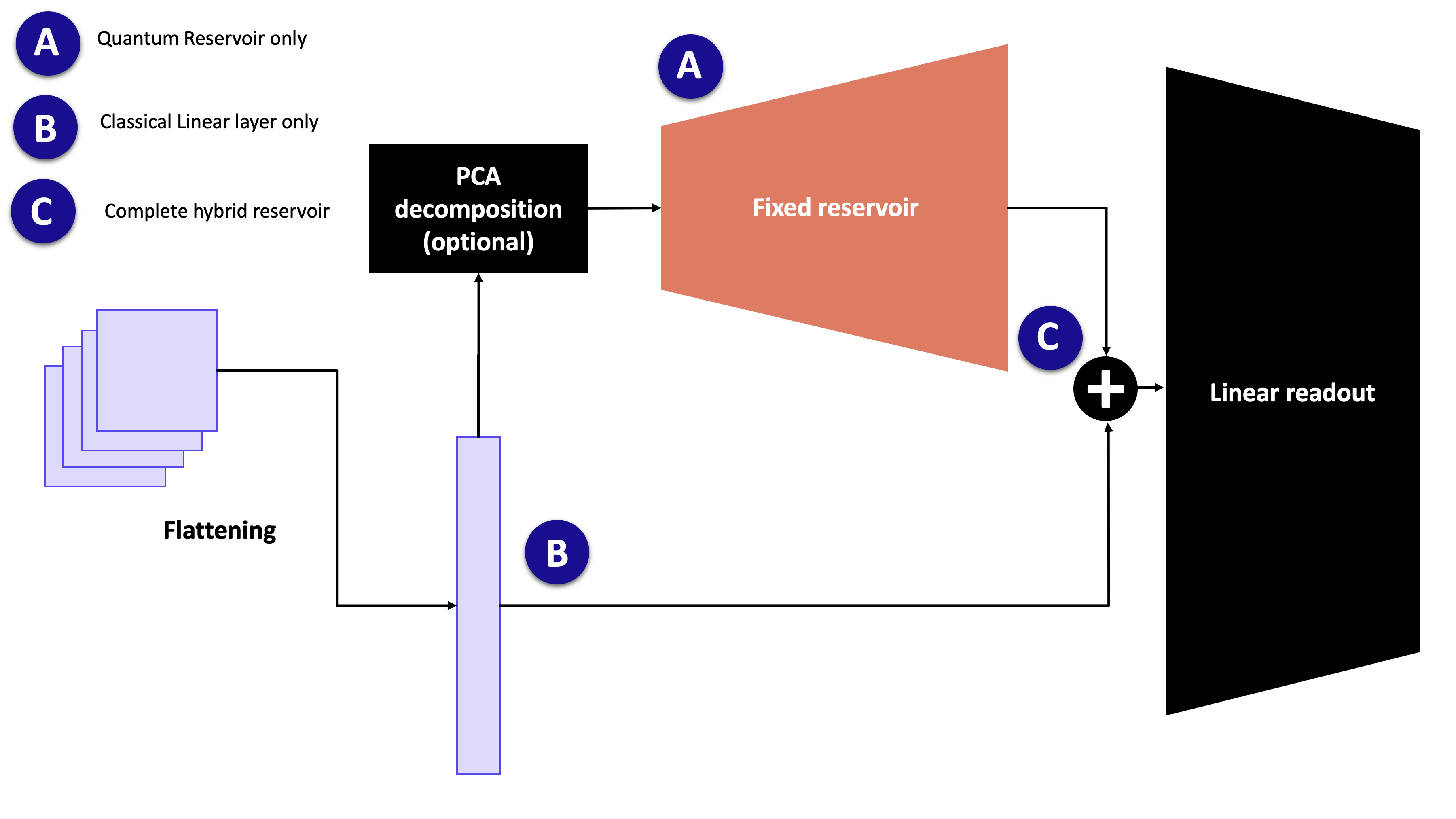
The model follows the same idea as classical reservoir computing: keep a rich feature map fixed, then train only a small readout. In MerLin, the feature map is a photonic circuit built from a Haar-random interferometer, phase encoding, the same interferometer again, and a measurement step.

Model structure

For an input vector \(x\), the classifier applies the following pipeline:

1. Optionally reduce the input dimension with a scikit-learn transformer such as sklearn.decomposition.PCA.

2. Scale the encoded features to the range used by the phase-shift encoder.

3. Run the frozen quantum reservoir:

   fixed interferometer U -> phase encoding E(x) -> fixed interferometer U -> measurement
   

4. Standardize the measured quantum features.

5. Concatenate the original input with the quantum features when concatenate=True.

6. Train a linear PyTorch readout on top of the resulting features.

Only the readout is trainable. The quantum layer parameters are frozen and are not returned by model.parameters().

Basic usage

The reservoir must be fitted before it can create readout datasets or predictions. fit_reservoir() fits the optional dimensionality reduction, learns input scaling, computes reservoir statistics, and initializes the readout width. make_dataset() then returns tensors that can be passed directly to a regular PyTorch training loop.

import torch
import torch.nn as nn
from sklearn.decomposition import PCA
from torch.utils.data import DataLoader

from merlin.models import ReservoirClassifier


seed = 7
device = torch.device("cpu")

model = ReservoirClassifier(
    in_features=X_train.shape[1],
    out_features=10,
    n_photons=3,
    reduction=PCA(
        n_components=12,
        svd_solver="randomized",
        random_state=seed,
    ),
    concatenate=True,
    cache=True,
    seed=seed,
    device=device,
    dtype=torch.float32,
)

model.fit_reservoir(X_train)
train_dataset = model.make_dataset(X_train, y_train)
train_loader = DataLoader(train_dataset, batch_size=128, shuffle=True)

criterion = nn.CrossEntropyLoss()
optimizer = torch.optim.Adam(model.parameters(), lr=1e-3)

for features, targets in train_loader:
    features = features.to(model.device, dtype=model.dtype)
    targets = targets.to(model.device)

    optimizer.zero_grad()
    logits = model(features)
    loss = criterion(logits, targets)
    loss.backward()
    optimizer.step()

test_logits = model.predict(X_test)
test_predictions = test_logits.argmax(dim=1)

This pattern is the same one used in the ReservoirClassifier notebook.

Choosing the input width

The number of encoded features determines the minimum circuit width. With no reduction, all input columns are encoded directly. This is useful for small datasets such as two-moons, where the reservoir can operate on the two original features.

For image datasets such as MNIST, reduce the flattened input before encoding:

model = ReservoirClassifier(
    in_features=784,
    out_features=10,
    n_photons=3,
    reduction=PCA(n_components=12, random_state=seed),
    concatenate=True,
    cache=True,
    seed=seed,
)

The default circuit uses n_components + 1 modes when a reduction is given, or in_features + 1 modes when it is not. Large direct inputs can therefore be expensive to simulate. Use a reduction step when the classical input has many features.

Readout inputs

The concatenate argument controls what the linear readout sees:

• concatenate=True trains on [x, r(x)], where x is the original raw input and r(x) is the standardized reservoir feature vector. This matches the protocol used by the ReservoirClassifier notebook.

• concatenate=False trains only on r(x).

The forward() method expects already transformed readout features. Use predict() when starting from raw inputs, because it runs the fitted preprocessing, the frozen reservoir, and the readout in the correct order.

Useful configuration hooks

Several reservoir-level choices are exposed through model.layer. Changing one of these rebuilds the frozen quantum layer and invalidates the fitted reservoir state, so call fit_reservoir() again afterwards.

Grouped measurements can reduce the quantum feature width before the readout:

from merlin import MeasurementStrategy, ModGrouping

model.layer.measurement_strategy = MeasurementStrategy.probs(
    grouping=ModGrouping(model.layer.output_size, model.out_features)
)
model.fit_reservoir(X_train)

The number of modes can be increased after construction:

model.layer.n_modes = 20
model.fit_reservoir(X_train)

n_modes cannot be smaller than the number of encoded input features plus one. The default reservoir input state also requires n_photons <= n_modes.

Noise can be attached through a Perceval noise model:

import perceval as pcvl

model.layer.noise = pcvl.NoiseModel(brightness=0.9)
model.fit_reservoir(X_train)

Caching

With cache=True, fit_reservoir() computes and stores the training-set quantum features. Reusing the same training matrix through make_dataset() then avoids recomputing the frozen photonic layer.

With cache=False, the model defers quantum feature computation until data is transformed. In that mode, transform the fitted training data first so the quantum feature standardization statistics are initialized before transforming new inputs.

Running the reservoir remotely

The readout always trains locally in PyTorch. Only the frozen reservoir feature extraction can be sent through a MerlinProcessor. Attach the processor to model.layer.processor before calling fit_reservoir():

import perceval as pcvl

from merlin import MerlinProcessor


pcvl.RemoteConfig.set_token(CLOUD_TOKEN)
remote_processor = pcvl.RemoteProcessor("sim:ascella")

model.layer.processor = MerlinProcessor(
    remote_processor=remote_processor,
    microbatch_size=32,
    timeout=3600.0,
)

model.fit_reservoir(X_train)
train_dataset = model.make_dataset(X_train, y_train)
test_logits = model.predict(X_test)

Use small per-class subsets first when running remotely, then increase the sample count once runtime and execution cost are clear.

Saving and loading

Use save() and load() to preserve the fitted preprocessing state, frozen reservoir state, cached features, and readout parameters:

model.save("reservoir_classifier.pt")
restored = ReservoirClassifier.load("reservoir_classifier.pt", device=device)

Reference

• API reference: merlin.models.reservoir_classifier module

• Full tutorial notebook: ReservoirClassifier on MNIST and Fashion-MNIST

ReservoirClassifier tutorial

MNIST and Fashion-MNIST workflows for the frozen reservoir classifier.

Quantum modelsReservoirMNISTClassification