Photonic QCNN

The QCNNClassifier is a ready-to-use photonic quantum convolutional neural network for square, single-channel image classification. It follows the photonic QCNN architecture with adaptive state injection introduced by Monbroussou et al. in Photonic Quantum Convolutional Neural Networks with Adaptive State Injection, Advanced Photonics, 7(6), 066012, 2025.

From an ML perspective, the model can be read as the quantum analogue of a compact CNN:

image values are amplitude-encoded into a two-register photonic state;
QConv layers apply local trainable filters with shared parameters;
QPool layers reduce the register size through measurement and state injection;
QDense mixes the remaining modes before a classical linear readout returns logits.

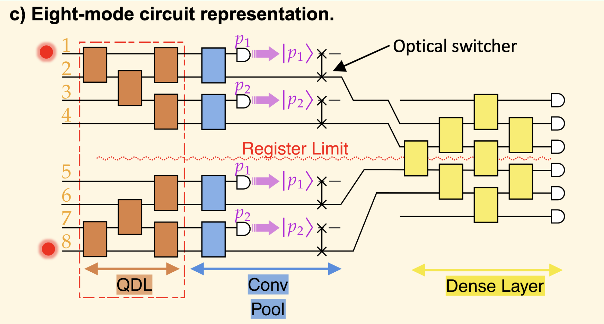
Photonic QCNN with adaptive state injection.

Image taken from the original paper.

Input Encoding

QCNNClassifier expects tensors with shape (batch_size, 1, height, width). The spatial shape must be square and must match the input_shape passed to the model.

Before the first layer, each image is converted to a normalized two-photon state vector. The row index is encoded in the first register and the column index is encoded in the second register:

\[|x\rangle = \frac{1}{\|x\|} \sum_{i=0}^{H-1} \sum_{j=0}^{W-1} x_{i,j}\, |e_i\rangle_\mathrm{row} |e_j\rangle_\mathrm{column}.\]

For a 4 x 4 image, the model uses 8 modes: 4 row modes and 4 column modes. A pixel x[i, j] becomes the amplitude of the Fock basis state with one photon in row mode i and one photon in column mode 4 + j. Basis states that do not respect this one-photon-per-register structure receive zero amplitude.

Architecture

The default architecture is:

QCNNClassifier(
    input_shape=(4, 4),
    num_classes=2,
    stages=None,
)

When stages is omitted, MerLin resolves it to:

[
    QCNNClassifier.QConv(kernel_size=2, stride=2),
    QCNNClassifier.QPool(kernel_size=2),
    QCNNClassifier.QDense(),
]

The executable model is a torch.nn.Sequential stored in model.layers. For the default architecture, its named modules are:

QConv_1 -> QPool_1 -> QDense -> Readout

QConv_1, QPool_1, and QDense are QuantumLayer instances. Readout is a torch.nn.Linear layer that maps the dense quantum probabilities to num_classes logits.

Quantum Convolution Layer

QCNNClassifier.QConv(kernel_size, stride) builds local trainable photonic filters. The layer works separately on the row and column registers, so no beam splitter directly mixes row modes with column modes during convolution.

For each register:

a sliding window covers kernel_size adjacent modes;
consecutive windows start stride modes apart;
each window is implemented by a down-and-up mesh of trainable beam splitters;
all windows in the same register share one trainable parameter.

The two registers use distinct trainable parameters:

px_first_register
px_second_register

This is the photonic equivalent of a classical convolutional filter with parameter sharing. It mixes local neighborhoods while preserving the two-register tensor-encoding structure. The layer returns amplitudes, not class scores, so later quantum layers can continue processing a state vector.

The convolution specification must satisfy:

kernel_size > 1;
stride > 0;
kernel_size <= current_register_size;
stride <= kernel_size.

Quantum Pooling Layer

QCNNClassifier.QPool(kernel_size) reduces the number of modes in each register. It is the state-injection layer of the photonic QCNN.

For every pooling window, MerLin measures the first mode. If the measured mode contains a photon, the post-processing reinserts one photon in the adjacent mode of the reduced register. Each valid measurement branch is then propagated through the remaining layers, and the branch logits are combined with their measurement probabilities.

For an input register of size d and a pooling kernel k, the current implementation reduces the register size to:

\[d - \frac{d}{k}.\]

With the default kernel_size=2, pooling halves each register. A 4 x 4 input encoded on 4 + 4 modes therefore reaches the dense layer with 2 + 2 modes.

The pooling specification must satisfy:

kernel_size > 1;
current_register_size % kernel_size == 0.

Quantum Dense Layer and Readout

QCNNClassifier.QDense() is mandatory and must be the final quantum stage. It builds a trainable beam-splitter mesh over all remaining modes, merging the row and column information before measurement.

The dense quantum layer returns Fock-basis probabilities. MerLin then applies a classical linear readout:

torch.nn.Linear(qdense.output_size, num_classes)

The model output is a tensor of logits with shape (batch_size, num_classes). Use the same loss functions as with regular PyTorch classifiers, for example torch.nn.CrossEntropyLoss.

Custom Stage Sequences

You can define a deeper QCNN by passing an explicit stage list:

from merlin.models import QCNNClassifier

model = QCNNClassifier(
    input_shape=(4, 4),
    num_classes=2,
    stages=[
        QCNNClassifier.QConv(kernel_size=2, stride=1),
        QCNNClassifier.QConv(kernel_size=2, stride=2),
        QCNNClassifier.QDense(),
    ],
)

Custom stages must follow these rules:

the list cannot be empty;
only QConv, QPool, and QDense stage objects are accepted;
exactly one QDense must appear, and it must be the last stage;
each QConv and QPool must be compatible with the current register size after previous pooling stages.

The resolved stage list is available through model.resolved_stages. The actual executable layers are available through model.layers.

Training Example

QCNNClassifier is a standard torch.nn.Module, so training uses the regular PyTorch workflow.

import torch

from merlin.models import QCNNClassifier

model = QCNNClassifier(input_shape=(4, 4), num_classes=2)
optimizer = torch.optim.Adam(model.parameters(), lr=1e-2)
loss_function = torch.nn.CrossEntropyLoss()

x = torch.rand(16, 1, 4, 4)
y = torch.randint(0, 2, (16,))

optimizer.zero_grad()
logits = model(x)
loss = loss_function(logits, y)
loss.backward()
optimizer.step()

Examples and References

QCNN API reference

Constructor, stage objects, layer API, and serialization helpers.

APIQCNNClassifierReference

Photonic QCNN reproduction

Paper reproduction for adaptive state injection in photonic QCNNs.

Reproduced paperQCNNVision

QCNNClassifier tutorial

Binary MNIST classification with the ready-to-use QCNN model.

TutorialMNISTClassification