Quantum Convolutional Neural Network for Classical Data Classification

Paper Information

Title: Quantum convolutional neural network for classical data classification

Authors: Tak Hur, Leeseok Kim, Daniel K. Park

Published: Quantum Machine Intelligence, Volume 4, Number 1, Page 3 (2022)

DOI: 10.1007/s42484-021-00061-x

Paper URL: arXiv:2108.00661

Original Repository: takh04/QCNN

Reproduction Status: ✅ Complete

Reproducer: Cassandre Notton (cassandre.notton@quandela.com)

Project Repository

Run the QCNN model

Complete code reproduction of QCNN_data_classification (quantum and classical baselines)

External LinkQCNNRepository

Abstract

This reproduction studies a quantum convolutional neural network (QCNN) pipeline for binary classical-image classification. The approach compresses MNIST-family inputs with PCA and applies a quantum pseudo-convolution stage before a classification head.

The reproduced setup includes two complementary workflows: a Merlin/Perceval implementation built with QuantumLayer and wrappers around the authors’ original TensorFlow/Keras QCNN code for benchmarking. The experiments compare quantum and classical pseudo-convolution variants under matched receptive-field settings.

Significance

The paper demonstrates that QCNN-style architectures can be adapted to classical data classification and can outperform simple classical baselines in selected settings. In this reproduction, the same idea is explored in a photonic workflow with explicit parameter/accuracy trade-offs across kernel modes, kernel sizes, strides, and number of kernels.

MerLin Implementation

Here, we implemented two main model variants:

• A photonic quantum convolution with parallel kernels

• A single Gaussian interferometer baseline

Core run options include quantum kernel topology (number, size and mode-count of kernels, stride), encoding strategy (angle or amplitude), and optimisation controls (steps, batch, seeds, learning rate).

How QuantumLayer is used in both models

The full implementation is in lib/merlin_reproduction.py. The two model paths use QuantumLayer differently:

1. SingleGI uses one global quantum layer directly on the PCA vector.

def build_single_gi_layer(n_modes, n_features, n_photons, reservoir_mode, state_pattern):
    circ = create_quantum_circuit(n_modes, n_features)
    trainable_prefixes = [] if reservoir_mode else ["theta"]
    input_state = StateGenerator.generate_state(n_modes, n_photons, StatePattern[state_pattern.upper()])
    return ML.QuantumLayer(
        input_size=n_modes,
        output_size=2,
        circuit=circ,
        trainable_parameters=trainable_prefixes,
        input_parameters=["px"],
        input_state=input_state,
        output_mapping_strategy=ML.OutputMappingStrategy.GROUPING,
    )

class SingleGI(nn.Module):
    def __init__(...):
        self.q = build_single_gi_layer(...)
    def forward(self, angles):
        return self.q(angles)

2. QConvModel uses one QuantumLayer per kernel and applies them to sliding PCA patches.

def _make_kernel() -> QuantumPatchKernel:
    q_layer = ML.QuantumLayer(
        input_size=kernel_modes,
        output_size=2,
        circuit=create_quantum_circuit(kernel_modes, args.kernel_size),
        trainable_parameters=["theta"],
        input_parameters=["px"],
        input_state=([1, 0] * (kernel_modes // 2) + [0]) if kernel_modes % 2 == 1 else [1, 0] * (kernel_modes // 2),
        output_mapping_strategy=ML.OutputMappingStrategy.GROUPING,
    )
    return QuantumPatchKernel(q_layer, required_inputs=kernel_required_inputs, patch_dim=args.kernel_size)

class QConvModel(nn.Module):
    def _apply_quantum_kernels(self, patches, num_windows, batch_size):
        patches_flat = patches.contiguous().view(-1, patches.size(-1))
        outputs = []
        for kernel in self.kernel_modules:
            y = kernel(patches_flat).view(batch_size, num_windows, -1)
            outputs.append(y)
        return torch.stack(outputs, dim=1).view(batch_size, -1)

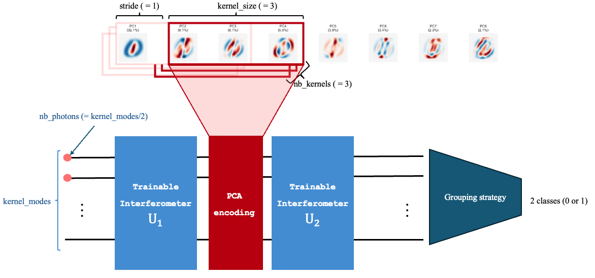
In short, SingleGI uses a single end-to-end photonic layer, while QConvModel reuses multiple photonic layers as learnable pseudo-convolution kernels over local PCA windows.

Photonic pseudo-convolution structure used by the MerLin QCNN reproduction.

Key Contributions Reproduced

Hybrid quantum/classical benchmark pipeline

• Reproduced the MNIST/FashionMNIST 0-vs-1 workflow with PCA-compressed inputs.

• Exposed matched quantum and classical pseudo-convolution baselines for direct comparison.

Hyperparameter and efficiency analysis

• Performed sweeps over kernel modes, number of kernels, kernel size, and stride.

• Reported both accuracy and parameter efficiency to identify Pareto-optimal settings.

Multiple encoding regimes

• Evaluated angle-encoding and amplitude-encoding variants.

• Measured robustness across PCA dimensions (8 and 16 components).

Implementation Details

The reproduction is designed to be straightforward to run from the command line. For full setup instructions, run commands, and implementation details, see: QCNN_data_classification README.

Experimental Results

Hyperparameter analysis (MNIST, PCA=8)

We performed a dedicated hyperparameter analysis for the quantum pseudo-convolution setup. The figure below summarizes overall validation accuracy across the tested quantum and classical model variants.

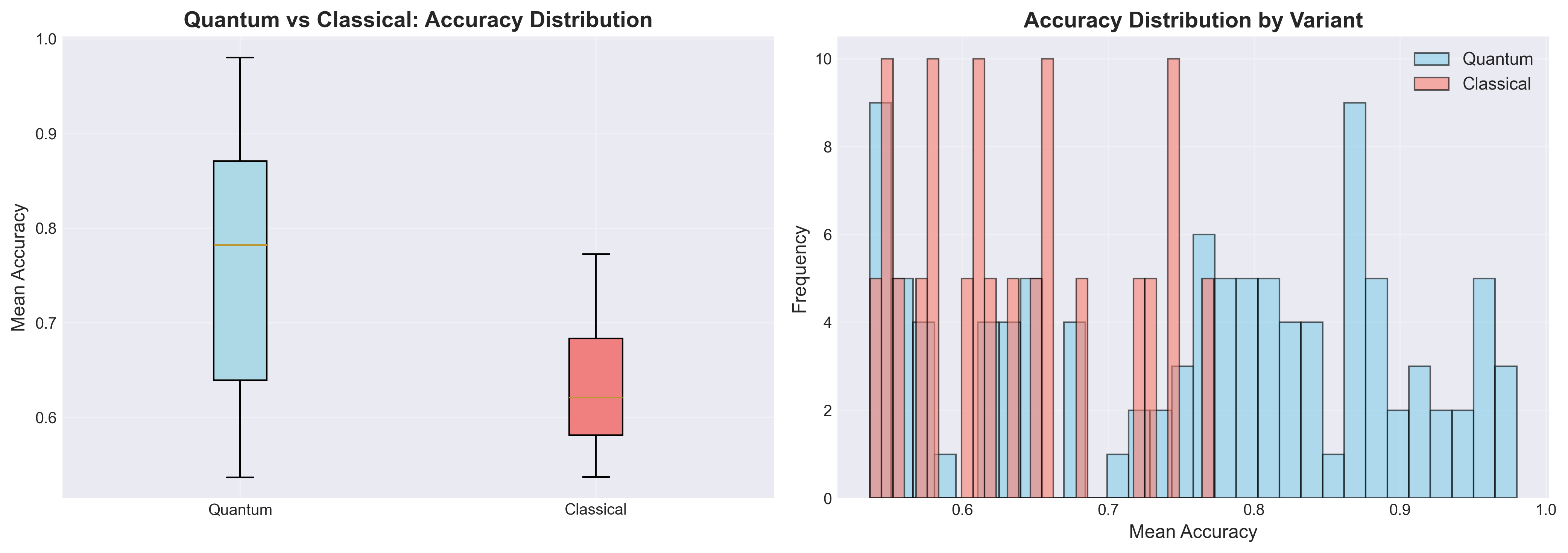
For full plots and detailed discussion, see the QCNN_data_classification README.

Angle-encoding benchmark (3 kernels, kernel size 3, stride 2)

Validation accuracy (mean ± std)

Model	8 PCA components	16 PCA components
Quantum convolution (830 trainable parameters) on MNIST	96.08 ± 3.64	80.11 ± 23.29
Quantum convolution (830 trainable parameters) on FashionMNIST	93.18 ± 1.20	82.75 ± 19.07
Classical convolution (32 trainable parameters) on MNIST	76.78 ± 11.16	72.84 ± 15.04
Classical convolution (32 trainable parameters) on FashionMNIST	81.35 ± 6.38	76.85 ± 23.14

Amplitude-encoding benchmark (6 kernel modes, 3 kernels, kernel size 3, stride 2)

Validation accuracy (mean ± std)

Model	8 PCA components	16 PCA components
Quantum convolution (128/176 trainable parameters) on MNIST	73.51 ± 14.07	66.89 ± 12.08
Quantum convolution (128/176 trainable parameters) on FashionMNIST	71.48 ± 12.53	74.13 ± 21.65

Training curves

All training-curve results are available in the QCNN_data_classification README.

Performance Analysis

Advantages

• The quantum pseudo-convolution reaches higher peak accuracies than the matched classical baseline in the reported angle-encoding setup.

• Hyperparameter sweeps provide actionable operating points balancing accuracy and parameter budget.

Current limitations

• Variance increases in some 16-PCA settings, indicating sensitivity to configuration and seed choice.

• Higher-performing quantum settings typically require substantially more trainable parameters than compact classical baselines.

Citation

@article{hur2022quantum,
  title={Quantum convolutional neural network for classical data classification},
  author={Hur, Tak and Kim, Leeseok and Park, Daniel K.},
  journal={Quantum Machine Intelligence},
  volume={4},
  number={1},
  pages={3},
  year={2022},
  publisher={Springer},
  doi={10.1007/s42484-021-00061-x}
}

---