Photonic Quantum Convolutional Neural Network with Adaptive State Injection
In this notebook, we will implement the Photonic QCNN from this paper and display its usage on the binary 8x8 MNIST classification task of differentiating 0 and 1. All of this will be done using MerLin, a photonic QML framework for the optimization of photonic circuits that was integrated with PyTorch for intuitive usage.
0. Imports
[20]:
import io
import math
import re
import sys
from collections.abc import Generator

import matplotlib.pyplot as plt
import numpy as np
import sympy as sp
import torch
import torch.nn.functional as F  # noqa: N812
from perceval import Circuit, GenericInterferometer, catalog
from sklearn.datasets import load_digits
from sklearn.model_selection import train_test_split
from torch import Tensor, nn, optim
from tqdm import trange

import merlin
from merlin import CircuitConverter
from merlin import build_slos_distribution_computegraph as build_slos_graph
from merlin.core.computation_space import ComputationSpace
1. Data
Function to fetch the 8x8 MNIST dataset from sklearn and choose the selected labels.
[21]:
def get_mnist(random_state, class_list=(0, 1)):
    """
    Get MNIST dataset reduced to certain labels.

    :param random_state
    :param class_list: List of labels to keep

    :return: x_train, x_test, y_train, y_test
    """
    mnist_x, mnist_y = load_digits(return_X_y=True)

    # Keep only selected classes
    mask = np.isin(mnist_y, class_list)
    mnist_x = mnist_x[mask]
    mnist_y = mnist_y[mask]

    # Train/test split
    mnist_x_train, mnist_x_test, mnist_y_train, mnist_y_test = train_test_split(
        mnist_x, mnist_y, test_size=200, random_state=random_state
    )
    # Since there are only 360 data points in this specific dataset with labels = 0 or 1, that implies that we will have 160 training points.

    # Reshape to 8×8 images
    mnist_x_train = mnist_x_train.reshape(-1, 8, 8)
    mnist_x_test = mnist_x_test.reshape(-1, 8, 8)

    return mnist_x_train, mnist_x_test, mnist_y_train, mnist_y_test


# Visualize an image from our training data
x_train, x_test, y_train, y_test = get_mnist(42)
plt.imshow(x_train[0], cmap="gray")
plt.axis("off")  # hide axes
plt.show()
print(f"With label: {y_train[0]}")

With label: 0
To convert the dataset arrays to data loaders.
[22]:
def convert_dataset_to_tensor(x_train, x_test, y_train, y_test):
    x_train = torch.tensor(x_train, dtype=torch.float32)
    x_test = torch.tensor(x_test, dtype=torch.float32)
    y_train = torch.tensor(y_train, dtype=torch.long)
    y_test = torch.tensor(y_test, dtype=torch.long)
    return x_train, x_test, y_train, y_test


def convert_tensor_to_loader(x_train, y_train, batch_size=6):
    train_dataset = torch.utils.data.TensorDataset(x_train, y_train)
    train_loader = torch.utils.data.DataLoader(
        train_dataset, batch_size=batch_size, shuffle=True
    )
    return train_loader
2. Model
All the following classes of which the complete photonic QCNN consists were implemented by Anthony Walsh.
We will start by defining 1 layer at a time. Let us start with the OneHotEncoder class which encodes each image to our circuit using amplitude encoding.
[23]:
class OneHotEncoder(nn.Module):
    """
    One Hot Encoder

    Converts an image `x` to density matrix in the One Hot Amplitude
    basis. For a given d by d image, the density matrix will be of
    size d^2 by d^2.
    """

    def __init__(self):
        super().__init__()

    def forward(self, x: Tensor) -> Tensor:
        if x.dim() == 3:
            x = x.unsqueeze(1)

        norm = torch.sqrt(torch.square(torch.abs(x)).sum(dim=(1, 2, 3)))
        x = x / norm.view(-1, 1, 1, 1)

        # Flatten each image and multiply by transpose to get density matrix
        x_flat = x.reshape(x.shape[0], -1)
        rho = x_flat.unsqueeze(2) @ x_flat.unsqueeze(1)
        rho = rho.to(torch.complex64)

        return rho

    def __repr__(self):
        return "OneHotEncoder()"
Second, we will define the convolutional layer called QConv2d and its parent abstract class AParametrizedLayer.
[24]:
class AQCNNLayer(nn.Module):
    """
    Abstract QCNN layer.

    Base class layer for inheriting functionality methods.

    Args:
        dims (tuple): Input dimensions into a parametrized layer.
    """

    def __init__(self, dims: tuple[int]):
        super().__init__()
        self.dims = dims
        self._training_params = []

        if dims[0] != dims[1]:
            raise NotImplementedError("Non-square images not supported yet.")

    def _check_input_shape(self, rho):
        """
        Checks that the shape of an input density matrix, rho matches
        the shape of the density matrix in the one hot encoding.
        """
        dim1 = rho.shape[1] ** 0.5
        dim2 = rho.shape[2] ** 0.5

        if not dim1.is_integer() or not dim2.is_integer():
            raise ValueError(
                "Shape of rho is not a valid. Please ensure that `rho` is a "
                "density matrix in the one-hot encoding space."
            )

        dim1, dim2 = int(dim1), int(dim2)

        if dim1 != self.dims[0] or dim2 != self.dims[1]:
            raise ValueError(
                "Input density matrix does not match specified dimensions. "
                f"Expected {self.dims}, received {(dim1, dim2)}. Please ensure"
                " that `rho` is a density matrix in the one-hot encoding space"
            )

    def _set_param_names(self, circuit):
        """
        Ensures that two different parametrized circuits have different
        perceval parameter names.
        """
        param_list = list(circuit.get_parameters())

        if not self._training_params:
            param_start_idx = 0
        else:
            # Take index from last parameter name
            param_start_idx = int(
                re.search(r"\d+", self._training_params[-1].name).group()
            )

        for i, p in enumerate(param_list):
            p.name = f"phi{i + param_start_idx + 1}"

        for _, comp in circuit:
            if hasattr(comp, "_phi"):
                param = comp.get_parameters()[0]
                param._symbol = sp.S(param.name)

        self._training_params.extend(param_list)


class QConv2d(AQCNNLayer):
    """
    Quantum 2D Convolutional layer.

    Args:
        dims: Input dimensions.
        kernel_size: Size of universal interferometer.
        stride: Stride of the universal interferometer across the
            modes.
    """

    def __init__(
        self,
        dims,
        kernel_size: int,
        stride: int = None,
    ):
        super().__init__(dims)
        self.kernel_size = kernel_size
        self.stride = kernel_size if stride is None else stride

        # Define filters
        filters = []
        for _ in range(2):
            filter = GenericInterferometer(
                kernel_size, catalog["mzi phase first"].generate
            )
            self._set_param_names(filter)
            filters.append(filter)

        # Create x and y registers
        self._reg_x = Circuit(dims[0], name="Conv X")
        self._reg_y = Circuit(dims[1], name="Conv Y")

        # Add filters with specified stride
        for i in range((dims[0] - kernel_size) // self.stride + 1):
            self._reg_x.add(self.stride * i, filters[0])

        for i in range((dims[1] - kernel_size) // self.stride + 1):
            self._reg_y.add(self.stride * i, filters[1])

        num_params_x = len(self._reg_x.get_parameters())
        num_params_y = len(self._reg_y.get_parameters())

        # Suppress unnecessary print statements from pcvl_pytorch
        original_stdout = sys.stdout
        sys.stdout = io.StringIO()
        try:
            # Build circuit graphs for the two registers separately.
            self._circuit_graph_x = CircuitConverter(
                self._reg_x, ["phi"], torch.float32
            )
            self._circuit_graph_y = CircuitConverter(
                self._reg_y, ["phi"], torch.float32
            )
        finally:
            sys.stdout = original_stdout

        # Create model parameters
        self.phi_x = nn.Parameter(2 * np.pi * torch.rand(num_params_x))
        self.phi_y = nn.Parameter(2 * np.pi * torch.rand(num_params_y))

    def forward(self, rho, adjoint=False):
        self._check_input_shape(rho)
        b = len(rho)

        # Compute unitary for the entire layer
        u_x = self._circuit_graph_x.to_tensor(self.phi_x)
        u_y = self._circuit_graph_y.to_tensor(self.phi_y)
        u = torch.kron(u_x, u_y)

        u = u.unsqueeze(0).expand(b, -1, -1)
        u_dag = u.transpose(1, 2).conj()

        # There is only one photon in each register, can apply the U directly.
        if not adjoint:
            u_rho = torch.bmm(u, rho)
            new_rho = torch.bmm(u_rho, u_dag)
        else:
            # Apply adjoint to rho
            u_dag_rho = torch.bmm(u_dag, rho)
            new_rho = torch.bmm(u_dag_rho, u)

        return new_rho

    def __repr__(self):
        return f"QConv2d({self.dims}, kernel_size={self.kernel_size}), stride={self.stride}"
Third, there is the pooling layer: QPooling.
[25]:
class QPooling(AQCNNLayer):
    """
    Quantum pooling layer.

    Reduce the size of the encoded image by the given kernel size.

    Args:
        dims: Input image dimensions.
        kernel_size: Dimension by which the image is reduced.
    """

    def __init__(self, dims: tuple[int], kernel_size: int):
        if dims[0] % kernel_size != 0:
            raise ValueError("Input dimensions must be divisible by the kernel size")

        super().__init__(dims)
        d = dims[0]
        k = kernel_size
        new_d = d // kernel_size

        self._new_d = new_d
        self.kernel_size = k

        # Create all index combinations at once
        x = torch.arange(d**2)
        y = torch.arange(d**2)

        # Our state is written in the basis: |e_f>|e_i>|e_j><e_h|<e_m|<e_n|

        # f, h represent the channel indices.
        # (Channels not included in this script)
        f = x // (d**2)
        h = y // (d**2)

        # Let i, j, m, n represent the one hot indices of the main register
        i = (x % (d**2)) // d
        j = (x % (d**2)) % d
        m = (y % (d**2)) // d
        n = (y % (d**2)) % d

        f_grid, h_grid = torch.meshgrid(f, h, indexing="ij")
        i_grid, m_grid = torch.meshgrid(i, m, indexing="ij")
        j_grid, n_grid = torch.meshgrid(j, n, indexing="ij")

        # Ensure that odd mode photon numbers match.
        match_odd1 = ((i_grid % k != 0) & (i_grid == m_grid)) | (i_grid % k == 0)
        match_odd2 = ((j_grid % k != 0) & (j_grid == n_grid)) | (j_grid % k == 0)

        # Ensure photon number in ancillae used for photon injection match
        inject_condition = (i_grid % k == m_grid % k) & (j_grid % k == n_grid % k)

        mask = inject_condition & match_odd1 & match_odd2
        mask_coords = torch.nonzero(mask, as_tuple=False)
        self._mask_coords = (mask_coords[:, 0], mask_coords[:, 1])

        # New one hot indices
        new_i = i_grid[mask] // k
        new_j = j_grid[mask] // k
        new_m = m_grid[mask] // k
        new_n = n_grid[mask] // k

        # New matrix coordinates
        self._new_x = new_i * new_d + new_j + f_grid[mask] * new_d**2
        self._new_y = new_m * new_d + new_n + h_grid[mask] * new_d**2

    def forward(self, rho):
        self._check_input_shape(rho)
        b = len(rho)

        b_indices = torch.arange(b).unsqueeze(1).expand(-1, len(self._new_x))
        b_indices = b_indices.reshape(-1)

        new_x = self._new_x.expand(b, -1).reshape(-1)
        new_y = self._new_y.expand(b, -1).reshape(-1)

        new_rho = torch.zeros(
            b, self._new_d**2, self._new_d**2, dtype=rho.dtype, device=rho.device
        )

        values = rho[:, self._mask_coords[0], self._mask_coords[1]].reshape(-1)
        new_rho.index_put_((b_indices, new_x, new_y), values, accumulate=True)

        return new_rho

    def __repr__(self):
        return f"QPooling({self.dims}, kernel_size={self.kernel_size})"
Fourth, there is the QDense layer which needs the functions generate_all_fock_states and compute_amplitude.
[26]:
def generate_all_fock_states(m, n) -> Generator:
    """
    Generate all possible Fock states for n photons and m modes.

    Args:
        m: Number of modes.
        n: Number of photons.

    Returns:
        Generator of tuples of each Fock state.
    """
    if n == 0:
        yield (0,) * m
        return
    if m == 1:
        yield (n,)
        return

    for i in range(n + 1):
        for state in generate_all_fock_states(m - 1, n - i):
            yield (i,) + state


def generate_all_fock_states_list(m, n, true_order=True) -> list:
    states_list = list(generate_all_fock_states(m, n))
    if true_order:
        states_list.reverse()
    return states_list
[27]:
# Cell 1: Fixed imports - add the missing import

# Cell 2: Fixed compute_amplitudes function
def compute_amplitudes(self, unitary: Tensor, input_state: list[int]) -> torch.Tensor:
    """
    Compute the amplitudes using the pre-built graph.

    Args:
        unitary (torch.Tensor): Single unitary matrix [m x m] or batch
            of unitaries [b x m x m]. The unitary should be provided in
            the complex dtype corresponding to the graph's dtype.
            For example: for torch.float32, use torch.cfloat;
            for torch.float64, use torch.cdouble.
        input_state (list[int]): Input_state of length self.m with
            self.n_photons in the input state

    Returns:
        Tensor: Output amplitudes associated with each Fock state.
    """
    # Add batch dimension
    if len(unitary.shape) == 2:
        unitary = unitary.unsqueeze(0)

    if any(n < 0 for n in input_state) or sum(input_state) == 0:
        raise ValueError("Photon numbers cannot be negative or all zeros")

    # Fix: Check computation_space instead of no_bunching
    if (
        hasattr(self, "computation_space")
        and self.computation_space is ComputationSpace.UNBUNCHED
    ):
        if not all(x in [0, 1] for x in input_state):
            raise ValueError(
                "Input state must be binary (0s and 1s only) in non-bunching mode"
            )

    batch_size, m, m2 = unitary.shape
    if m != m2 or m != self.m:
        raise ValueError(
            f"Unitary matrix must be square with dimension {self.m}x{self.m}"
        )

    # Check dtype to match the complex dtype used for the graph building
    if unitary.dtype != self.complex_dtype:
        raise ValueError(
            f"Unitary dtype {unitary.dtype} doesn't match the expected complex"
            f" dtype {self.complex_dtype} for the graph built with dtype"
            f" {self.dtype}. Please provide a unitary with the correct dtype "
            f"or rebuild the graph with a compatible dtype."
        )

    idx_n = []
    norm_factor_input = torch.tensor(1.0, dtype=self.dtype, device=unitary.device)

    for i, count in enumerate(input_state):
        for c in range(count):
            norm_factor_input *= c + 1
            idx_n.append(i)

            if hasattr(self, "index_photons"):
                bounds1 = self.index_photons[len(idx_n) - 1][1]
                bounds2 = self.index_photons[len(idx_n) - 1][0]
                if (i > bounds1) or (i < bounds2):
                    raise ValueError(
                        f"Input state photons must be bounded by {self.index_photons}"
                    )

    # Get device from unitary
    device = unitary.device

    # Initial amplitude - need to add superposition dimension for layer_compute_batch
    amplitudes = torch.ones(
        (batch_size, 1, 1),  # [batch_size, initial_states, num_inputs]
        dtype=self.complex_dtype,
        device=device,
    )

    # Fix: Use layer_compute_batch with vectorized operations instead of layer_functions
    # Import the actual function (this should be available from slos_torchscript)
    from merlin.pcvl_pytorch.slos_torchscript import layer_compute_batch

    # Apply each layer using the vectorized operations
    for layer_idx in range(len(self.vectorized_operations)):
        p = [idx_n[layer_idx]]  # Wrap in list as layer_compute_batch expects list[int]
        sources, destinations, modes = self.vectorized_operations[layer_idx]

        amplitudes = layer_compute_batch(
            unitary,
            amplitudes,
            sources,
            destinations,
            modes,
            p,
        )

    # Remove the superposition dimension since we only have one input component
    amplitudes = amplitudes.squeeze(2)

    # Store for debugging
    self.prev_amplitudes = amplitudes

    # Normalize the amplitudes
    self.norm_factor_output = self.norm_factor_output.to(device=device)
    amplitudes = amplitudes * torch.sqrt(self.norm_factor_output.unsqueeze(0))
    amplitudes = amplitudes / torch.sqrt(norm_factor_input)

    return amplitudes


# Cell 3: Fixed QDense class initialization to use correct SLOS graph
class QDense(AQCNNLayer):
    """
    Quantum Dense layer.

    Expects an input density matrix in the One Hot Amplitude basis and
    performs SLOS to return the output density matrix in the whole Fock
    space.

    Args:
        dims (tuple[int]): Input image dimensions.
        m (int | list[int]): Size of the dense layers placed in
            succession. If `None`, a single universal dense layer is
            applied.
    """

    def __init__(self, dims, m: int | list[int] = None, device=None):
        super().__init__(dims)

        self.device = device
        m = m if m is not None else sum(dims)
        self.m = [m]

        # Construct circuit and circuit graph
        self._training_params = []

        self.circuit = Circuit(max(self.m))
        for m in self.m:
            gi = GenericInterferometer(m, catalog["mzi phase first"].generate)
            self._set_param_names(gi)
            self.circuit.add(0, gi)

        # Suppress unnecessary print statements
        original_stdout = sys.stdout
        sys.stdout = io.StringIO()
        try:
            self._circuit_graph = CircuitConverter(self.circuit, ["phi"], torch.float32)
        finally:
            sys.stdout = original_stdout

        # Set up input states & SLOS graphs
        self._input_states = [
            tuple(int(i == x) for i in range(dims[0]))
            + tuple(int(i == y) for i in range(dims[1]))
            for x in range(dims[1])
            for y in range(dims[0])
        ]

        # Fix: Build SLOS graph without expecting return_distributions parameter
        self._slos_graph = build_slos_graph(
            m=max(self.m),
            n_photons=2,
            device=self.device,
            # Don't pass computation_space here - use default
        )

        # Monkey-patch the compute_amplitudes method
        self._slos_graph.compute_amplitudes = lambda u, s: compute_amplitudes(
            self._slos_graph, u, s
        )

        # Create and register model parameters
        num_params = len(self._training_params)
        self.phi = nn.Parameter(2 * np.pi * torch.rand(num_params))

    def forward(self, rho):
        self._check_input_shape(rho)
        b = len(rho)

        # Run SLOS & extract amplitudes
        unitary = self._circuit_graph.to_tensor(self.phi)

        # Compute amplitudes for each basis state
        amplitudes = torch.stack([
            self._slos_graph.compute_amplitudes(unitary, basis_state)
            for basis_state in self._input_states
        ])

        # Handle batch dimension properly
        if amplitudes.dim() == 3 and amplitudes.shape[1] == 1:
            amplitudes = amplitudes.squeeze(1)  # Remove batch dimension if size 1

        u_evolve = amplitudes.T

        # Amplitudes constitute evolution operator
        u_evolve = u_evolve.expand(b, -1, -1)
        u_evolve_dag = u_evolve.transpose(1, 2).conj()

        # Extract upper triangular & divide diagonal by 2
        upper_rho = torch.triu(rho)
        diagonal_mask = torch.eye(rho.size(-1), dtype=torch.bool)
        upper_rho[..., diagonal_mask] /= 2

        # U rho U dagger for hermitian rho
        inter_rho1 = torch.bmm(u_evolve, upper_rho)
        inter_rho = torch.bmm(inter_rho1, u_evolve_dag)

        new_rho = inter_rho + inter_rho.transpose(1, 2).conj()
        return new_rho

    def __repr__(self):
        m = self.m[0] if len(self.m) == 1 else self.m
        return f"QDense({self.dims}, m={m})"
Fifth, we define the measurement class: Measure.
[28]:
class Measure(nn.Module):
    """
    Measurement operator.

    Assumes input is written in Fock basis and extracts diagonal.

    If one would like to perform a partial measurement, the following
    params can be specified.

    Args:
        m (int): Total number of modes in-device. Default: None.
        n (int): Number of photons in-device. Default: 2.
        subset (int): Number of modes being measured. Default: None.
    """

    def __init__(self, m: int = None, n: int = 2, subset: int = None):
        super().__init__()
        self.m = m
        self.n = n
        self.subset = subset

        if subset is not None:
            all_states = generate_all_fock_states_list(m, n)
            reduced_states = []
            for i in range(n + 1):
                reduced_states += generate_all_fock_states_list(subset, i)
            self.reduced_states_len = len(reduced_states)

            self.indices = torch.tensor([
                reduced_states.index(state[:subset]) for state in all_states
            ])

    def forward(self, rho):
        b = len(rho)
        probs = torch.abs(rho.diagonal(dim1=1, dim2=2))

        if self.subset is not None:
            indices = self.indices.unsqueeze(0).expand(b, -1)
            probs_output = torch.zeros(
                (b, self.reduced_states_len), device=probs.device, dtype=probs.dtype
            )
            """probs_output = torch.zeros(
                indices.shape, device=probs.device, dtype=probs.dtype
            )"""
            probs_output.scatter_add_(dim=1, index=indices, src=probs)
            return probs_output

        return probs

    def __repr__(self):
        if self.subset is not None:
            return f"Measure(m={self.m}, n={self.n}, subset={self.subset})"
        else:
            return "Measure()"
Finally, we define our entire model, PQCNN, and its helper functions.
[29]:
def marginalize_photon_presence(keys, probs):
    """
    keys: List of tuples, each tuple of length num_modes (e.g., (0, 1, 0, 2))
    probs: Tensor of shape (N, num_keys), with requires_grad=True

    Returns:
        Tensor of shape (N, num_modes) with the marginal probability
        that each mode has at least one photon.
    """
    device = probs.device
    keys_tensor = torch.tensor(
        keys, dtype=torch.long, device=device
    )  # shape: (num_keys, num_modes)
    keys_tensor.shape[1]

    # Create mask of shape (num_modes, num_keys)
    # Each mask[i] is a binary vector indicating which Fock states have >=1 photon in mode i
    mask = (keys_tensor >= 1).T  # shape: (num_modes, num_keys)

    # Convert to float to allow matrix multiplication
    mask = mask.float()

    # Now do: (N, num_keys) @ (num_keys, num_modes) → (N, num_modes)
    marginalized = probs @ mask.T  # shape: (N, num_modes)
    return marginalized


def generate_partial_fock_states(subset, n, m):
    """
    Generate all the possible Fock state considering a subset of modes.

    Args:
    :param subset: Number of modes to consider. Has to be smaller or equal to m (number of modes)
    :param n: Number of photons
    :param m: Total number of modes
    :return: List of all possible Fock states considering the subset of modes
    """
    reduced_states = []
    # Account for when subset == m or subset + 1 == m. There cannot have 1 or 0 photon
    for i in range(max(0, subset - m + n), n + 1):
        reduced_states += generate_all_fock_states_list(subset, i)
    return reduced_states


def partial_measurement_output_size(subset: int, n: int, total_modes: int) -> int:
    """
    Compute number of possible measurement outcomes when measuring a subset
    of modes in Fock space, constrained by total photon number.

    Args:
        subset (int): Number of measured modes
        n (int): Total number of photons
        total_modes (int): Total number of modes (m)

    Returns:
        int: Number of reduced Fock states consistent with measurement
    """
    if subset == total_modes:
        # Full measurement: all photons must be in measured modes
        return math.comb(subset + n - 1, n)
    else:
        # Partial measurement: sum over all valid photon counts in measured modes
        return sum(math.comb(subset + i - 1, i) for i in range(n + 1))
[30]:
class PQCNN(nn.Module):
    def __init__(
        self, dims, measure_subset, output_proba_type, output_formatting, num_classes=2
    ):
        super().__init__()
        self.num_modes_end = dims[0]
        self.num_modes_measured = (
            measure_subset if measure_subset is not None else dims[0]
        )

        self.one_hot_encoding = OneHotEncoder()
        self.conv2d = QConv2d(dims, kernel_size=2, stride=2)
        self.pooling = QPooling(dims, kernel_size=2)
        self.dense = QDense((int(dims[0] / 2), int(dims[1] / 2)))
        self.measure = Measure(m=dims[0], n=2, subset=measure_subset)

        self.qcnn = nn.Sequential(
            self.one_hot_encoding, self.conv2d, self.pooling, self.dense, self.measure
        )

        # Output dimension of the QCNN
        # Depends on whether we consider the probability of each Fock state or of each mode separately
        self.output_proba_type = output_proba_type
        if output_proba_type == "state":
            if measure_subset is not None:
                qcnn_output_dim = partial_measurement_output_size(
                    self.num_modes_measured, 2, self.num_modes_end
                )
            else:
                states = list(generate_all_fock_states(self.num_modes_end, 2))
                qcnn_output_dim = len(states)
            print(f"Number of Fock states: {qcnn_output_dim}")

        elif output_proba_type == "mode":
            if measure_subset is not None:
                qcnn_output_dim = measure_subset
            else:
                qcnn_output_dim = self.num_modes_end  # Number of modes
            # qcnn_output_dim = self.num_modes_end
        else:
            raise NotImplementedError(
                f"Output probability type {output_proba_type} not implemented"
            )
        self.qcnn_output_dim = qcnn_output_dim

        # Output mapping strategy
        if output_formatting == "Train_linear":
            self.output_mapping = nn.Linear(qcnn_output_dim, num_classes)
        elif output_formatting == "No_train_linear":
            self.output_mapping = nn.Linear(qcnn_output_dim, num_classes)
            self.output_mapping.weight.requires_grad = False
            self.output_mapping.bias.requires_grad = False
        elif output_formatting == "Lex_grouping":
            self.output_mapping = merlin.utils.grouping.LexGrouping(
                qcnn_output_dim, num_classes
            )
        elif output_formatting == "Mod_grouping":
            self.output_mapping = merlin.utils.grouping.ModGrouping(
                qcnn_output_dim, num_classes
            )
        else:
            raise NotImplementedError

        if measure_subset is not None:
            self.keys = generate_partial_fock_states(
                measure_subset, 2, self.num_modes_end
            )
        else:
            self.keys = generate_all_fock_states(self.num_modes_end, 2)
        # self.keys = generate_all_fock_states_list(self.num_modes_end, 2)

    def forward(self, x):
        probs = self.qcnn(x)

        if self.output_proba_type == "mode":
            probs = marginalize_photon_presence(self.keys, probs)

        output = self.output_mapping(probs)
        output = output * 66

        return output
3. Training
Train the PQCNN with the CrossEntropyLoss using Adam optimizer.
[31]:
def train_model(model, train_loader, x_train, x_test, y_train, y_test):
    """Train a single model and return training history"""
    optimizer = torch.optim.Adam(model.parameters(), lr=0.1, weight_decay=0.001)
    scheduler = optim.lr_scheduler.ExponentialLR(optimizer, gamma=0.9)
    loss_fn = nn.CrossEntropyLoss()

    loss_history = []
    train_acc_history = []
    test_acc_history = []

    # Initial accuracy
    with torch.no_grad():
        output_train = model(x_train)
        pred_train = torch.argmax(output_train, dim=1)
        train_acc = (pred_train == y_train).float().mean().item()

        output_test = model(x_test)
        pred_test = torch.argmax(output_test, dim=1)
        test_acc = (pred_test == y_test).float().mean().item()

        train_acc_history.append(train_acc)
        test_acc_history.append(test_acc)

    # Training loop
    for _epoch in trange(20, desc="Training epochs"):
        for _batch_idx, (images, labels) in enumerate(train_loader):
            optimizer.zero_grad()
            output = model(images)
            loss = loss_fn(output, labels)
            loss.backward()
            optimizer.step()
            loss_history.append(loss.item())

        # Evaluate accuracy
        with torch.no_grad():
            output_train = model(x_train)
            pred_train = torch.argmax(output_train, dim=1)
            train_acc = (pred_train == y_train).float().mean().item()

            output_test = model(x_test)
            pred_test = torch.argmax(output_test, dim=1)
            test_acc = (pred_test == y_test).float().mean().item()

            train_acc_history.append(train_acc)
            test_acc_history.append(test_acc)
        scheduler.step()
    return {
        "loss_history": loss_history,
        "train_acc_history": train_acc_history,
        "test_acc_history": test_acc_history,
        "final_train_acc": train_acc,
        "final_test_acc": test_acc,
    }
Set up hyperparameters.
[32]:
# Hyperparameters
measure_subset = 2  # Number of modes to measure

output_proba_type = "mode"  # ['state', 'mode']
# MerLin default is 'state'. If set to 'mode', the circuit output has the following format:
# [proba of photon in mode 1, proba of photon in mode 2, ... , proba of photon in mode m]
# If set to 'state', the circuit output has the following form:
# [proba of Fock state 1, proba of Fock state 2, ... , proba of Fock state N]

output_formatting = "Mod_grouping"  # ['Train_linear', 'No_train_linear', 'Lex_grouping', 'Mod_grouping']
# Format of the mapping from circuit output to number of labels. The only one that has trainable parameters is 'Train_linear'.

random_states = [42, 123, 456, 789, 999]
Multiple runs to do.
[33]:
all_results = {}

for i, random_state in enumerate(random_states):
    print(f"About to start experiment {i + 1}/5")
    x_train, x_test, y_train, y_test = get_mnist(random_state=random_state)
    x_train, x_test, y_train, y_test = convert_dataset_to_tensor(
        x_train, x_test, y_train, y_test
    )
    train_loader = convert_tensor_to_loader(x_train, y_train)
    dims = (8, 8)

    pqcnn = PQCNN(dims, measure_subset, output_proba_type, output_formatting)
    num_params = sum(p.numel() for p in pqcnn.parameters() if p.requires_grad)
    print(f"Model has {num_params} trainable parameters")
    print(f"Output of circuit has size {pqcnn.qcnn_output_dim}")

    results = train_model(pqcnn, train_loader, x_train, x_test, y_train, y_test)
    print(
        f"MNIST - Final train: {results['final_train_acc']:.4f}, test: {results['final_test_acc']:.4f}"
    )
    print(f"Experiment {i + 1}/5 completed")
    all_results[f"run_{i}"] = results
About to start experiment 1/5
Model has 60 trainable parameters
Output of circuit has size 2
Training epochs: 100%|██████████| 20/20 [01:49<00:00, 5.45s/it]
MNIST - Final train: 1.0000, test: 0.9950
Experiment 1/5 completed
About to start experiment 2/5
Model has 60 trainable parameters
Output of circuit has size 2
Training epochs: 100%|██████████| 20/20 [01:31<00:00, 4.58s/it]
MNIST - Final train: 1.0000, test: 0.9900
Experiment 2/5 completed
About to start experiment 3/5
Model has 60 trainable parameters
Output of circuit has size 2
Training epochs: 100%|██████████| 20/20 [00:56<00:00, 2.84s/it]
MNIST - Final train: 1.0000, test: 1.0000
Experiment 3/5 completed
About to start experiment 4/5
Model has 60 trainable parameters
Output of circuit has size 2
Training epochs: 100%|██████████| 20/20 [00:49<00:00, 2.48s/it]
MNIST - Final train: 1.0000, test: 1.0000
Experiment 4/5 completed
About to start experiment 5/5
Model has 60 trainable parameters
Output of circuit has size 2
Training epochs: 100%|██████████| 20/20 [00:56<00:00, 2.82s/it]
MNIST - Final train: 1.0000, test: 0.9950
Experiment 5/5 completed
4. Results
Display training metrics and print overall results
[34]:
# Save summary statistics
summary = {}
num_runs = len(all_results)
train_accs = [all_results[f"run_{i}"]["final_train_acc"] for i in range(num_runs)]
test_accs = [all_results[f"run_{i}"]["final_test_acc"] for i in range(num_runs)]

summary = {
    "train_acc_mean": np.mean(train_accs),
    "train_acc_std": np.std(train_accs),
    "test_acc_mean": np.mean(test_accs),
    "test_acc_std": np.std(test_accs),
    "train_accs": train_accs,
    "test_accs": test_accs,
}

# Create training plots for each dataset
fig, axes = plt.subplots(1, 3, figsize=(18, 5))
colors = ["blue", "red", "green", "orange", "purple"]

# Plot loss history for this dataset
ax_loss = axes[0]
for run_idx in range(num_runs):
    loss_history = all_results[f"run_{run_idx}"]["loss_history"]
    ax_loss.plot(
        loss_history,
        color=colors[run_idx],
        alpha=1,
        linewidth=2,
        label=f"Run {run_idx + 1}",
    )
ax_loss.set_title("MNIST - Training Loss")
ax_loss.set_xlabel("Training Steps")
ax_loss.set_ylabel("Loss")
ax_loss.legend()
ax_loss.grid(True, alpha=0.3)

# Plot train accuracy for this dataset
ax_train = axes[1]
for run_idx in range(num_runs):
    train_acc_history = all_results[f"run_{run_idx}"]["train_acc_history"]
    epochs = range(len(train_acc_history))
    ax_train.plot(
        epochs,
        train_acc_history,
        color=colors[run_idx],
        alpha=1,
        linewidth=2,
        label=f"Run {run_idx + 1}",
    )
ax_train.set_title("MNIST - Training Accuracy")
ax_train.set_xlabel("Epochs")
ax_train.set_ylabel("Accuracy")
ax_train.legend()
ax_train.grid(True, alpha=0.3)
ax_train.set_ylim(0, 1)

# Plot test accuracy for this dataset
ax_test = axes[2]
for run_idx in range(num_runs):
    test_acc_history = all_results[f"run_{run_idx}"]["test_acc_history"]
    epochs = range(len(test_acc_history))
    ax_test.plot(
        epochs,
        test_acc_history,
        color=colors[run_idx],
        alpha=1,
        linewidth=2,
        label=f"Run {run_idx + 1}",
    )
ax_test.set_title("MNIST - Test Accuracy")
ax_test.set_xlabel("Epochs")
ax_test.set_ylabel("Accuracy")
ax_test.legend()
ax_test.grid(True, alpha=0.3)
ax_test.set_ylim(0, 1)

plt.tight_layout()
plt.show()

# Print summary
print("\nSummary Results:")
print("=" * 50)
print("Binary MNIST 0 vs 1:")
print(
    f"  Train Accuracy: {summary['train_acc_mean']:.3f} ± {summary['train_acc_std']:.3f}"
)
print(
    f"  Test Accuracy:  {summary['test_acc_mean']:.3f} ± {summary['test_acc_std']:.3f}"
)
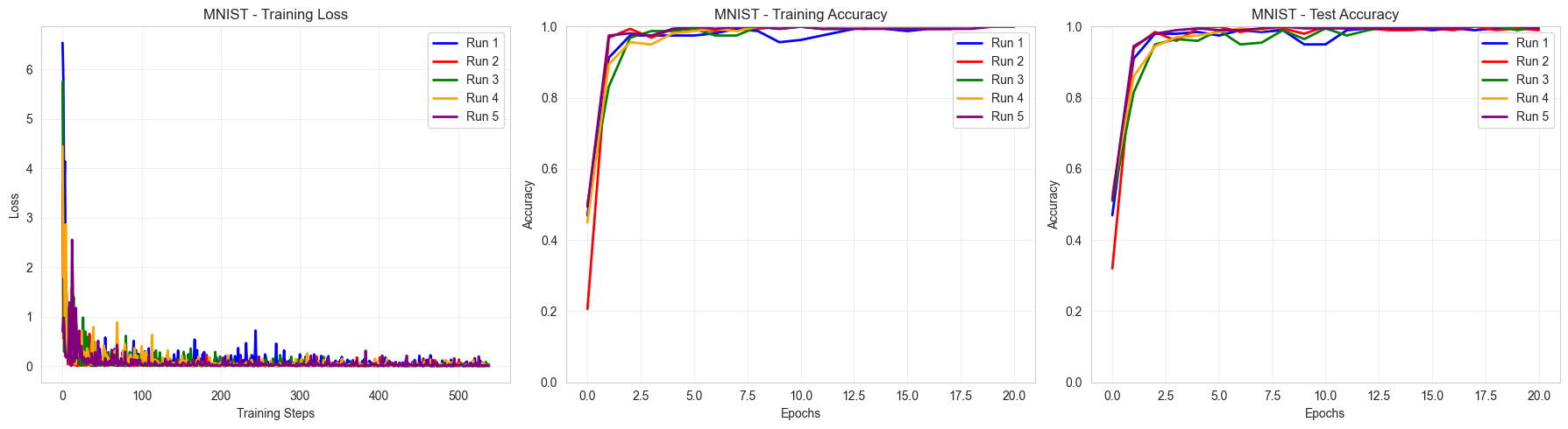
Summary Results:
==================================================
Binary MNIST 0 vs 1:
  Train Accuracy: 1.000 ± 0.000
  Test Accuracy:  0.996 ± 0.004
As we can see, our PQCNN easily and consistently manages to classify 8x8 MNIST images between labels 0 and 1.
5. Classical comparison
Let us now compare these results with the ones from a classical CNN of comparable number of parameters. We first need to define this CNN:
[35]:
class SmallCNN(nn.Module):
    def __init__(self):
        super().__init__()
        # Conv layer: in_channels=1 (grayscale), out_channels=1, kernel=3
        self.conv1 = nn.Conv2d(1, 2, kernel_size=3)  # 1*2*3*3 + 2 bias = 20 params
        # output of size (6, 6, 2)

        self.pool = nn.MaxPool2d(2, 2)
        # output of size (3, 3, 2)

        # Fully connected: after conv + pool, output size is 2 × 3 × 3 = 18
        self.fc1 = nn.Linear(18, 2)  # 18*2 + 2 biases = 38 params → we'll adjust

        # Total number of params: 58

    def forward(self, x):
        x = F.relu(self.conv1(x))
        x = self.pool(x)
        x = torch.flatten(x, 1)  # Flatten except batch dim
        x = self.fc1(x)
        return x
Let us redefine the training function:
[36]:
def train_model(model, train_loader, x_train, x_test, y_train, y_test):
    """Train a single model and return training history"""
    optimizer = torch.optim.Adam(
        model.parameters(), lr=0.1, weight_decay=0.001, betas=(0.7, 0.9)
    )
    # scheduler = optim.lr_scheduler.ExponentialLR(optimizer, gamma=0.9)
    loss_fn = nn.CrossEntropyLoss()

    loss_history = []
    train_acc_history = []
    test_acc_history = []

    # Initial accuracy
    with torch.no_grad():
        output_train = model(x_train)
        pred_train = torch.argmax(output_train, dim=1)
        train_acc = (pred_train == y_train).float().mean().item()

        output_test = model(x_test)
        pred_test = torch.argmax(output_test, dim=1)
        test_acc = (pred_test == y_test).float().mean().item()

        train_acc_history.append(train_acc)
        test_acc_history.append(test_acc)

    # Training loop
    for _epoch in trange(100, desc="Training epochs"):
        for _batch_idx, (images, labels) in enumerate(train_loader):
            optimizer.zero_grad()
            output = model(images)
            loss = loss_fn(output, labels)
            loss.backward()
            optimizer.step()
            loss_history.append(loss.item())

        # Evaluate accuracy
        with torch.no_grad():
            output_train = model(x_train)
            pred_train = torch.argmax(output_train, dim=1)
            train_acc = (pred_train == y_train).float().mean().item()

            output_test = model(x_test)
            pred_test = torch.argmax(output_test, dim=1)
            test_acc = (pred_test == y_test).float().mean().item()

            train_acc_history.append(train_acc)
            test_acc_history.append(test_acc)
        # scheduler.step()
    return {
        "loss_history": loss_history,
        "train_acc_history": train_acc_history,
        "test_acc_history": test_acc_history,
        "final_train_acc": train_acc,
        "final_test_acc": test_acc,
    }
Then we run the experiments:
[37]:
all_results = {}

for i, random_state in enumerate(random_states):
    print(f"About to start experiment {i + 1}/5")
    x_train, x_test, y_train, y_test = get_mnist(random_state=random_state)
    x_train, x_test, y_train, y_test = convert_dataset_to_tensor(
        x_train, x_test, y_train, y_test
    )
    x_train = x_train.unsqueeze(dim=1)
    x_test = x_test.unsqueeze(dim=1)
    train_loader = convert_tensor_to_loader(x_train, y_train)
    dims = (8, 8)

    classical_cnn = SmallCNN()
    num_params = sum(p.numel() for p in classical_cnn.parameters() if p.requires_grad)
    print(f"Model has {num_params} trainable parameters")

    results = train_model(classical_cnn, train_loader, x_train, x_test, y_train, y_test)
    print(
        f"MNIST - Final train: {results['final_train_acc']:.4f}, test: {results['final_test_acc']:.4f}"
    )
    print(f"Experiment {i + 1}/5 completed")
    all_results[f"run_{i}"] = results
About to start experiment 1/5
Model has 58 trainable parameters
Training epochs: 100%|██████████| 100/100 [00:16<00:00, 6.15it/s]
MNIST - Final train: 1.0000, test: 0.9800
Experiment 1/5 completed
About to start experiment 2/5
Model has 58 trainable parameters
Training epochs: 100%|██████████| 100/100 [00:15<00:00, 6.29it/s]
MNIST - Final train: 1.0000, test: 0.9800
Experiment 2/5 completed
About to start experiment 3/5
Model has 58 trainable parameters
Training epochs: 100%|██████████| 100/100 [00:14<00:00, 6.88it/s]
MNIST - Final train: 1.0000, test: 0.9900
Experiment 3/5 completed
About to start experiment 4/5
Model has 58 trainable parameters
Training epochs: 100%|██████████| 100/100 [00:14<00:00, 6.94it/s]
MNIST - Final train: 0.9937, test: 1.0000
Experiment 4/5 completed
About to start experiment 5/5
Model has 58 trainable parameters
Training epochs: 100%|██████████| 100/100 [00:17<00:00, 5.87it/s]
MNIST - Final train: 1.0000, test: 0.9950
Experiment 5/5 completed
Visualize the results
[38]:
# Save summary statistics
summary = {}
num_runs = len(all_results)
train_accs = [all_results[f"run_{i}"]["final_train_acc"] for i in range(num_runs)]
test_accs = [all_results[f"run_{i}"]["final_test_acc"] for i in range(num_runs)]

summary = {
    "train_acc_mean": np.mean(train_accs),
    "train_acc_std": np.std(train_accs),
    "test_acc_mean": np.mean(test_accs),
    "test_acc_std": np.std(test_accs),
    "train_accs": train_accs,
    "test_accs": test_accs,
}

# Create training plots for each dataset
fig, axes = plt.subplots(1, 3, figsize=(18, 5))
colors = ["blue", "red", "green", "orange", "purple"]

# Plot loss history for this dataset
ax_loss = axes[0]
for run_idx in range(num_runs):
    loss_history = all_results[f"run_{run_idx}"]["loss_history"]
    ax_loss.plot(
        loss_history,
        color=colors[run_idx],
        alpha=1,
        linewidth=2,
        label=f"Run {run_idx + 1}",
    )
ax_loss.set_title("MNIST - Training Loss")
ax_loss.set_xlabel("Training Steps")
ax_loss.set_ylabel("Loss")
ax_loss.legend()
ax_loss.grid(True, alpha=0.3)

# Plot train accuracy for this dataset
ax_train = axes[1]
for run_idx in range(num_runs):
    train_acc_history = all_results[f"run_{run_idx}"]["train_acc_history"]
    epochs = range(len(train_acc_history))
    ax_train.plot(
        epochs,
        train_acc_history,
        color=colors[run_idx],
        alpha=1,
        linewidth=2,
        label=f"Run {run_idx + 1}",
    )
ax_train.set_title("MNIST - Training Accuracy")
ax_train.set_xlabel("Epochs")
ax_train.set_ylabel("Accuracy")
ax_train.legend()
ax_train.grid(True, alpha=0.3)
ax_train.set_ylim(0, 1)

# Plot test accuracy for this dataset
ax_test = axes[2]
for run_idx in range(num_runs):
    test_acc_history = all_results[f"run_{run_idx}"]["test_acc_history"]
    epochs = range(len(test_acc_history))
    ax_test.plot(
        epochs,
        test_acc_history,
        color=colors[run_idx],
        alpha=1,
        linewidth=2,
        label=f"Run {run_idx + 1}",
    )
ax_test.set_title("MNIST - Test Accuracy")
ax_test.set_xlabel("Epochs")
ax_test.set_ylabel("Accuracy")
ax_test.legend()
ax_test.grid(True, alpha=0.3)
ax_test.set_ylim(0, 1)

plt.tight_layout()
plt.show()

# Print summary
print("\nSummary Results:")
print("=" * 50)
print("Binary MNIST 0 vs 1:")
print(
    f"  Train Accuracy: {summary['train_acc_mean']:.3f} ± {summary['train_acc_std']:.3f}"
)
print(
    f"  Test Accuracy:  {summary['test_acc_mean']:.3f} ± {summary['test_acc_std']:.3f}"
)
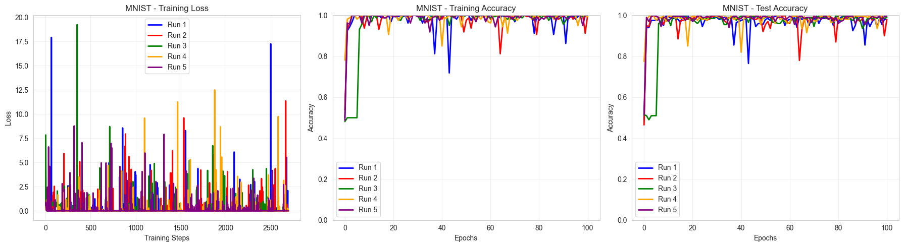
Summary Results:
==================================================
Binary MNIST 0 vs 1:
  Train Accuracy: 0.999 ± 0.003
  Test Accuracy:  0.989 ± 0.008
With 58 parameters classically (versus the 60 quantum parameters), we end up with an equivalent performance in terms of accuracy. The non-smoothness of the classical training differentiates the two but more hyperparameters optimization could solve this issue.