Noisy simulations with SLOS

Why use noisy simulations?

Current photonic processors are noisy. A model trained only with ideal simulation can therefore learn from output probabilities that are cleaner than the probabilities produced by the hardware.

Merlin can add the main Quandela hardware noise sources to SLOS simulations through pcvl.NoiseModel. This makes the training distribution closer to the distribution expected from the QPU.

The user-facing rule is simple: noisy simulations return probabilities. They do not return ideal amplitudes, because the noise model changes probability distributions.

Run a noisy QuantumLayer

Create a pcvl.NoiseModel and attach it either to the pcvl.Experiment or directly to QuantumLayer.

import perceval as pcvl
import torch

import merlin as ML

circuit = pcvl.Circuit(3)
circuit.add((0, 1), pcvl.BS())
circuit.add(0, pcvl.PS(pcvl.P("px")))
circuit.add((1, 2), pcvl.BS())

noise = pcvl.NoiseModel(
    brightness=0.85,
    transmittance=0.9,
    indistinguishability=0.95,
    g2=0.02,
    g2_distinguishable=False,
    phase_imprecision=0.01,
    phase_error=0.02,
)

layer = ML.QuantumLayer(
    input_size=1,
    circuit=circuit,
    input_parameters=["px"],
    input_state=[1, 1, 1],
    noise=noise,
    n_phase_error_samples=10,
    measurement_strategy=ML.MeasurementStrategy.probs(
        computation_space=ML.ComputationSpace.FOCK
    ),
)

x = torch.rand(3, 1)
probabilities = layer(x)

The same noise model can be stored in the experiment instead:

experiment = pcvl.Experiment(circuit, noise=noise)

layer = ML.QuantumLayer(
    input_size=1,
    experiment=experiment,
    input_parameters=["px"],
    input_state=[1, 1, 1],
    n_phase_error_samples=10,
    measurement_strategy=ML.MeasurementStrategy.probs(
        computation_space=ML.ComputationSpace.FOCK
    ),
)

If both the experiment and the layer define a noise model, they must be the same.

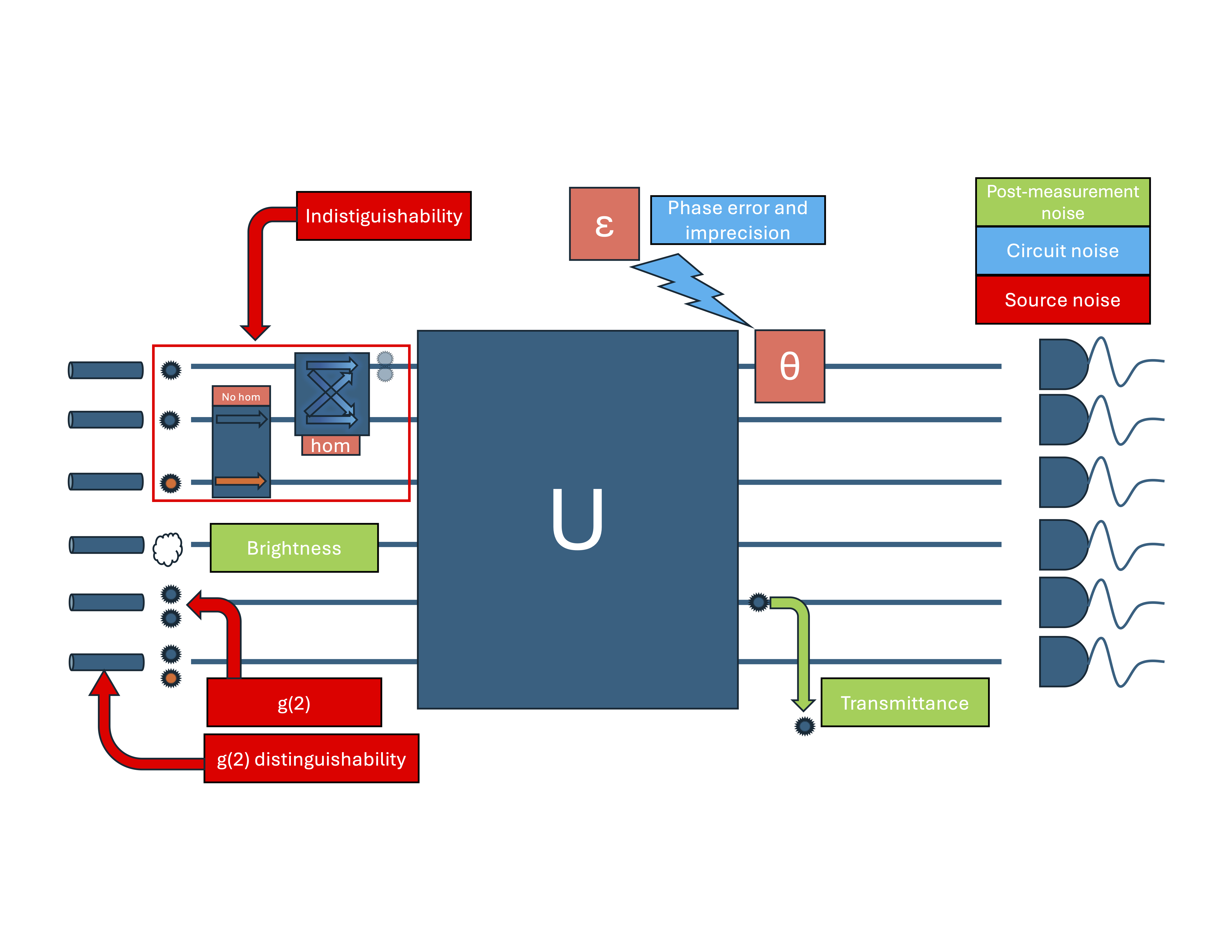
Supported noise sources

The active hardware noise sources are split into three groups.

Noise types summary on the interferometer

Noise source	Parameter	Default	Practical effect
Brightness	`brightness`	`1.0`	The source sometimes emits no photon.
Transmittance	`transmittance`	`1.0`	A photon can be lost while crossing the processor.
Phase imprecision	`phase_imprecision`	`0.0`	Phase shifter values are rounded to a finite resolution.
Phase error	`phase_error`	`0.0`	Phase shifter values receive a random perturbation.
Indistinguishability	`indistinguishability`	`1.0`	Photons can become partially distinguishable and interfere less.
Multi-photon emission	`g2`	`0.0`	A source can emit an extra photon.
Multi-photon distinguishability	`g2_distinguishable`	Perceval default	Extra photons from `g2` can be treated as distinguishable.

Post-measurement noise

Brightness and transmittance both model missing photons. Their product is the probability that one expected photon is emitted and survives the processor.

Use lower values when you want the output distribution to include states with fewer photons than the ideal input state.

noise = pcvl.NoiseModel(
    brightness=0.8,
    transmittance=0.9,
)

For an input state with n photons, the output basis can contain sectors from 0 to n photons.

Circuit noise

Circuit noise changes the phases used by the interferometer.

phase_imprecision models finite phase-shifter resolution. If phase_imprecision=0.1, the phase used in the forward pass is the nearest multiple of 0.1 radians.

noise = pcvl.NoiseModel(phase_imprecision=0.1)

phase_error models random phase fluctuations. For each phase-error sample, Merlin perturbs the phase shifters, computes the probability distribution, and then averages the sampled probability distributions.

noise = pcvl.NoiseModel(phase_error=0.02)

layer = ML.QuantumLayer(
    input_size=1,
    circuit=circuit,
    input_parameters=["px"],
    input_state=[1, 0, 1],
    noise=noise,
    n_phase_error_samples=20,
    measurement_strategy=ML.MeasurementStrategy.probs(
        computation_space=ML.ComputationSpace.FOCK
    ),
)

Set torch.manual_seed before calling the layer if you need reproducible phase-error samples.

Source noise

Source noise changes the photon state before it enters the interferometer.

Indistinguishability

indistinguishability is the probability that emitted photons are identical enough to interfere. The perfect value is 1.0. Smaller values reduce quantum interference and move the result toward a classical distribution.

A simple Hong-Ou-Mandel experiment shows the effect. Two indistinguishable photons entering a 50:50 beam splitter bunch together: both photons leave in the same mode.

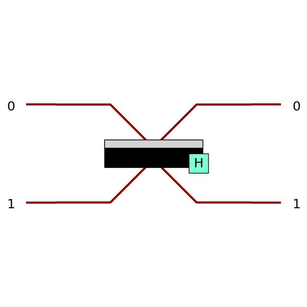
import perceval as pcvl

import merlin as ML

circuit = pcvl.Circuit(2)
circuit.add((0, 1), pcvl.BS.H())

layer = ML.QuantumLayer(
    input_size=0,
    circuit=circuit,
    input_state=[1, 1],
    measurement_strategy=ML.MeasurementStrategy.probs(
        computation_space=ML.ComputationSpace.FOCK
    ),
)

probabilities = layer()

for state, probability in zip(layer.output_keys, probabilities.flatten()):
    print(f"{state}: {probability}")

Output:

(2, 0): 0.49999991059303284
(1, 1): 0.0
(0, 2): 0.49999991059303284

With fully distinguishable photons, the photons no longer bunch perfectly:

layer = ML.QuantumLayer(
    input_size=0,
    circuit=circuit,
    input_state=[1, 1],
    noise=pcvl.NoiseModel(indistinguishability=0.0),
    measurement_strategy=ML.MeasurementStrategy.probs(
        computation_space=ML.ComputationSpace.FOCK
    ),
)

probabilities = layer()

Output:

(2, 0): 0.25
(1, 1): 0.5
(0, 2): 0.25

Multi-photon emission

The g2 value is correlated to the probability that a source emits two photons instead of one. Mathematically, it is defined by \(g(2)=\frac{\langle n(n-1)\rangle}{\langle n \rangle^2}\). Here, since we only analyze the probability that a second photon is emitted and not higher-order emissions, we can define p as the probability that two photons are emitted: \(p=\frac{1-g(2)-\sqrt{1-2g(2)}}{2g(2)}\). So a g(2) of 0.5 corresponds to the case where all generated photons are duplicated.

Merlin treats each intended input photon as one g2 source slot. If the input state is bunched, each photon in the occupied mode may be duplicated. For example, in the \(\ket{2,0,0}\) input state, the \(\ket{2,0,0}\), \(\ket{3,0,0}\), and \(\ket{4,0,0}\) states are simulated.

This noise can change the output type considerably when running the forward method of a QuantumLayer. Indeed, if an extra photon is generated, the interferometer simulation is performed in a completely different Fock space. To illustrate this, we use the same simple circuit used to describe indistinguishability noise and the same \(\ket{1,1}\) input state.

import perceval as pcvl
import merlin as ml

#Creating the BS circuit
circuit = pcvl.Circuit(2)
circuit.add([0, 1], pcvl.BS.H())

#Running the circuit
layer = ml.QuantumLayer(
    input_size=0,
    circuit=circuit,
    input_state=[1, 1],
    measurement_strategy=ml.MeasurementStrategy.probs(
        computation_space=ml.ComputationSpace.FOCK
    ),
    noise=pcvl.NoiseModel(g2=0.25),
)
output = layer()

#Printing the probabilities
for key, prob in zip(layer.output_keys, output.flatten()):
    print(f"Output probability of state {key} is {prob}")

Output:

Output probability of state (2, 0) is 0.1348033845424652
Output probability of state (1, 0) is 0.019606785848736763
Output probability of state (0, 0) is 0.1348033845424652
Output probability of state (1, 1) is 0.016084961593151093
Output probability of state (0, 1) is 0.0053616538643836975
Output probability of state (0, 2) is 0.0053616538643836975
Output probability of state (3, 0) is 0.016084961593151093
Output probability of state (2, 1) is 0.0006899359868839383
Output probability of state (1, 2) is 0.0
Output probability of state (0, 3) is 0.00045995728578418493
Output probability of state (4, 0) is 0.0
Output probability of state (3, 1) is 0.0006899359868839383
Output probability of state (2, 2) is 0.2285533845424652
Output probability of state (1, 3) is 0.2285533845424652
Output probability of state (0, 4) is 0.2089466005563736

We observe that the output is a large torch.Tensor. Indeed, because the space analyzed by a quantum interferometer depends on the number of input photons (the Fock space dimension for n photons and m modes is defined by \(\binom{m+n-1}{n}\)). Thus, g2 noise simulations explore a larger space and are handled differently in the output of the QuantumLayer’s forward method. Photon loss and detectors are applied to each sector independently.

The default value of the g2 parameter of the NoiseModel is 0.0. This is the case where no extra photons are ever generated.

Rules and limitations

Noisy simulations currently have these constraints:

Use probs().
Use the SLOS backend.
Keep return_object=False.
Do not use partial measurement with active noise.
Use FOCK for source noise, because source noise can add photons, remove photons, and create bunched states.
With g2 > 0, interpret columns through layer.output_keys because the flattened output can contain several photon-number sectors.

Use detectors to match hardware outputs

Current Quandela hardware uses threshold detectors. A threshold detector reports whether at least one photon was detected in a mode; it does not report the exact number of photons in that mode.

Use pcvl.Detector objects in the experiment when you want the simulated output space to match this detector behavior.

import perceval as pcvl

import merlin as ML

circuit = pcvl.Circuit(2)
circuit.add((0, 1), pcvl.BS.H())

experiment = pcvl.Experiment(m_circuit=circuit)
experiment.detectors[0] = pcvl.Detector.threshold()
experiment.detectors[1] = pcvl.Detector.threshold()

layer = ML.QuantumLayer(
    input_size=0,
    experiment=experiment,
    input_state=[1, 1],
    noise=pcvl.NoiseModel(g2=0.25, brightness=0.5),
    measurement_strategy=ML.MeasurementStrategy.probs(
        computation_space=ML.ComputationSpace.FOCK
    ),
)

probabilities = layer()

print(layer.output_size)
for state, probability in zip(layer.output_keys, probabilities.flatten()):
    print(f"{state}: {probability}")

Output:

4
(1, 0): 0.38013163208961487
(0, 0): 0.2089466005563736
(1, 1): 0.030790047720074654
(0, 1): 0.38013163208961487

Further details

This page describes the noise sources from a user point of view. For formulas, Monte Carlo details, source-noise mixtures, and memory considerations, see Noisy Simulations.