Noisy Simulations
This page describes how Merlin implements noisy SLOS simulations. For a
practical introduction to the available noise parameters and a first
QuantumLayer example, see
Noisy simulations with SLOS.
Noisy Simulation Implementation
SLOS normally propagates amplitudes. Active source noise and stochastic phase error are represented as probability mixtures, so Merlin computes and combines probability distributions for those cases. The implementation details below describe where each noise family enters the computation.
Brightness and Transmittance
Brightness and transmittance are implemented in the same workflow. Merlin first
computes the ideal probability tensor for the fixed n-photon, m-mode
Fock space, then applies photon survival as a transition matrix over the output
probabilities. The survival probability for each photon is the product of
brightness and transmittance.
Algorithm
Compute
\[l = \sum_{i=0}^{n} \dim(\mathcal{F}_{m,i})\]where \(\mathcal{F}_{m,i}\) denotes the Fock space of
mmodes andiphotons.Initialize the transition matrix as a tensor of zeros with shape
\[(\dim(\mathcal{F}_{m,n}), l)\]For each basis state in the
(m, n)Fock space:For each possible output state:
Compute the probability
\[\binom{n}{n_{\mathrm{survived}}} (b t)^{n_{\mathrm{survived}}} (1-b t)^{n-n_{\mathrm{survived}}}\]where:
\(n_{\mathrm{survived}}\) is the number of photons that survive,
\(b\) is the source brightness,
\(t\) is the transmittance.
Assign the probability to the appropriate column of the transition matrix using the output state’s corresponding index and key.
Return the completed transition matrix.
The possible output states are all of the possible combinations of losing photons in the basis state.
For g2 simulations, the photon loss algorithm is applied per n-photon sector at the output of the simulation. Indeed, the transition matrix is different for each sector. After this noise is applied, the probabilities are reclassified and returned as a large tensor.
Phase Error and Imprecision
Circuit phase noise is applied while Merlin builds the differentiable circuit unitary.
phase_imprecision is deterministic. Each phase shifter value is quantized to
the nearest multiple of phase_imprecision during the forward pass:
where \(\Delta \phi\) is phase_imprecision. This is nearest-grid
rounding, not truncation. Merlin uses torch.round for this operation, so
exact half-step ties follow PyTorch’s rounding behavior. For example, if the
commanded phase is \(\pi/8\) and phase_imprecision is \(\pi/4\),
then \(\phi / \Delta \phi = 0.5\) and the quantized phase is 0. Values
slightly above \(\pi/8\) quantize to \(\pi/4\). Merlin uses a
straight-through estimator, so gradients still flow through the commanded phase
value even though the forward pass uses the quantized phase.
phase_error is stochastic. For each Monte Carlo sample, Merlin draws a fresh
Torch random perturbation from Uniform(-phase_error, phase_error) for every
phase shifter, builds one unitary, computes probabilities, then averages the
probability distributions. Amplitudes are not averaged. Use
torch.manual_seed(...) to make the sampled perturbations reproducible.
Coherent and incoherent error
A coherent error is represented by a unitary transformation. It preserves the
phase relations between components of a quantum state, so amplitudes can still
interfere before they are converted to probabilities. In Merlin, deterministic
phase_imprecision is coherent within a forward pass: it changes the phase
values used to build the unitary, but the circuit is still evaluated as one
unitary.
phase_error is a stochastic coherent error at the sample level. Each Monte
Carlo sample draws one perturbed unitary and evaluates the quantum evolution
coherently for that unitary. Merlin then converts that sample’s output
amplitudes to probabilities and averages the probabilities over all sampled
unitaries:
This is different from averaging amplitudes or unitaries first:
Merlin does not use this second expression for phase_error.
For example, consider two sampled output states:
Each sampled state has probability \(1/2\) on \(|10\rangle\) and probability \(1/2\) on \(|01\rangle\), so averaging probabilities keeps the 50/50 distribution. Averaging amplitudes first cancels the \(|01\rangle\) component. If that averaged amplitude vector is then renormalized, it becomes \(|10\rangle\), giving probability 1 on \(|10\rangle\) and probability 0 on \(|01\rangle\). This is not the Monte Carlo probability mixture used by Merlin.
An incoherent error is represented as a classical mixture of alternatives. The relative phases between alternatives are not used for interference; Merlin combines probabilities, not amplitudes. Source noise is handled this way. For a tensor input state interpreted as a superposition, source-noise simulations propagate each active input basis state independently and combine the resulting probability distributions with weights \(|c_i|^2\).
The practical consequence is:
with circuit phase noise only, a tensor input superposition remains coherent inside each sampled unitary;
with source noise, tensor input components are treated as an incoherent mixture over basis states;
with
phase_error, the final reported distribution is an incoherent Monte Carlo average of probability distributions, even though each sampled unitary is evaluated coherently.
When both circuit phase noises are active, Merlin first quantizes the phase and then samples the stochastic perturbation around the quantized value:
where \(e\) is phase_error. If phase_imprecision is inactive, Merlin
uses \(\phi + \epsilon\). If phase_error is inactive, Merlin uses only
the deterministic quantized phase.
The n_phase_error_samples constructor parameter controls how many sampled
unitaries are averaged when active phase_error is present. If omitted,
Merlin uses 1 sample. Runtime scales roughly linearly with this value when
phase_error > 0. When source noise or g2 is also active, the cost is
multiplicative: each phase-error sample runs the full source-noise mixture, so
the worst-case runtime is roughly
n_phase_error_samples * n_active_input_states * SLOS.
Suggested values:
1for Perceval-like stochastic circuit sampling.5to10for quick expected-noise estimates.50to100for validation studies.200or more for production or publication results.
The parameter is ignored when phase_error is None or 0.0.
import math

import perceval as pcvl
import torch
import merlin as ML

circuit = pcvl.Circuit(2)
circuit.add((0, 1), pcvl.BS.H())
circuit.add(0, pcvl.PS(pcvl.P("phi")))
circuit.add((0, 1), pcvl.BS.H())

layer = ML.QuantumLayer(
    input_size=0,
    circuit=circuit,
    input_state=[1, 0],
    n_photons=1,
    trainable_parameters=["phi"],
    noise=pcvl.NoiseModel(
        phase_imprecision=math.pi / 4,
        phase_error=0.1,
    ),
    n_phase_error_samples=50,
    measurement_strategy=ML.MeasurementStrategy.probs(
        computation_space=ML.ComputationSpace.FOCK
    ),
)

torch.manual_seed(42)
probs_1 = layer()
torch.manual_seed(42)
probs_2 = layer()

assert torch.allclose(probs_1, probs_2)
In this example, a commanded trainable phase equal to math.pi / 8 would be
quantized to 0 before the stochastic perturbation is added, because it lies
exactly halfway between the 0 and math.pi / 4 grid points and
torch.round(0.5) returns 0.
Indistinguishability
This noise is implemented using the one-bad-bit (OBB) principle first introduced in Merlin in this reproduced paper. Indeed, since distinguishable photons can be tracked independently, each of those independent photons can be simulated separately. This implementation is done in the NoisySLOSComputeGraph class. Here are the main steps:
Algorithm
Create a
SLOSComputeGraphobject formmodes and photon numbers ranging from1ton, wherenis the number of photons in the input state.For each possible configuration of distinguishable photons:
Run a single-photon SLOS simulation for each distinguishable photon.
Run a SLOS simulation for all remaining photons, treating them as indistinguishable.
Convolve the resulting output distributions.
Multiply the convolved distribution by
\[p^{\,n-n_{\mathrm{dist}}} (1-p)^{\,n_{\mathrm{dist}}}\]where:
\(p\) is the photon indistinguishability,
\(n\) is the number of photons in the input state,
\(n_{\mathrm{dist}}\) is the number of distinguishable photons.
Sum the weighted distributions into the output tensor.
Return the resulting output tensor.
The combinations of possible distinguishable photons are simply the ways of choosing 0 to n photons from the input state.
g2 and g2 distinguishable
These noises build on the NoisySLOSComputeGraph class to create the NoisyG2SLOSComputeGraph object. Indeed, the noisy simulation must be performed for multiple input states with photon duplication. Here are the main implementation steps.
The g2 value is converted to the probability \(p\) that one source
emits an extra photon:
Only the no-extra-photon and one-extra-photon cases are modeled for each input photon. Higher-order emissions from the same source are not included.
Algorithm
Create a
NoisySLOSComputeGraphobject formmodes andiphotons, withiranging fromnto2n.If
g2_distinguishableisTrue, create aSLOSComputeGraphobject formmodes and a single photon.Generate all possible photon-addition vectors. These are the vectors for all possible sequences of duplicated photons.
For example, for the input state
[1,1,0]:[[0,0,0]]— no duplicated photons.[[1,0,0], [0,1,0]]— one duplicated photon.[[1,1,0]]— both photons duplicated.
Group the vectors according to the number of added photons.
For each group corresponding to
iadded photons:For each photon-addition vector:
If
g2_distinguishableisTrue:Run the original input state on the
SLOSComputeGraphwithnphotons.Run the single-photon SLOS computation for each added photon.
Convolve the resulting output distributions.
Otherwise:
Run the augmented input state on the
SLOSComputeGraphwithn+iphotons.
Multiply the resulting distribution by
\[p^{i}(1-p)^{n-i}\]where
pis the probability that two photons are emitted andnis the photon number of the desired input state.
Combine all distributions into the tensor representing the
n_iphoton sector.
Return the probability distribution for each photon sector.
Noisy Simulations Limitations
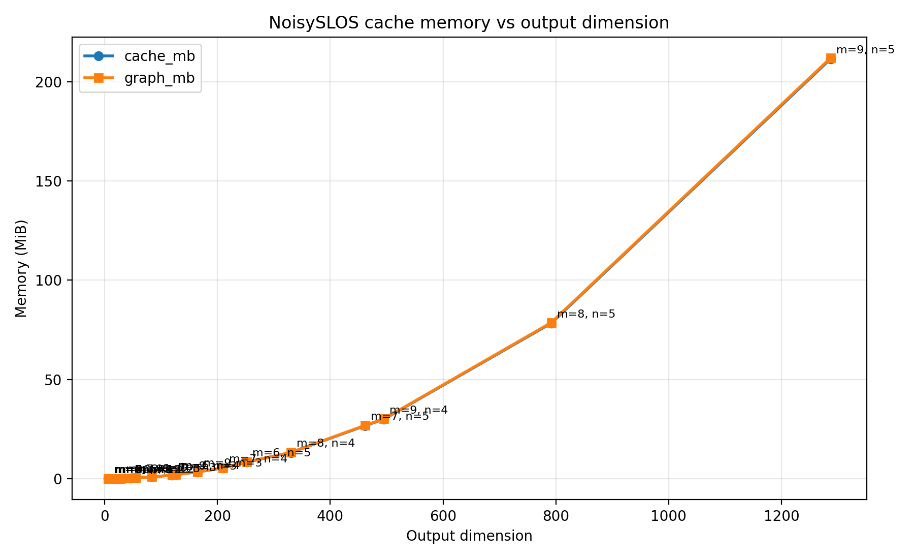
Noisy simulations are significantly less efficient than ideal ones. You can profile the memory requirements of noisy simulations with source noise using the benchmark script: ../../benchmarks/benchmark_noisy_slos_cache_memory.py.
Memory and computational complexity grow significantly with the number of modes and photons. For example, a 5-photon 2-mode circuit requires around 200 MB, while a 20-mode 3-photon experiment requires around 3 GB. This is only for indistinguishable photons. Memory requirements are even greater for g2 simulations. To profile memory consumption in your specific use case, run the benchmark script with:
python benchmarks/benchmark_noisy_slos_cache_memory.py --modes 6 7 8 9 --photons 1 2 3 4 5 --backward
Here is an example of the output graph of this run.
The public API constraints are listed in Noisy simulations with SLOS. The implementation reason is that Merlin does not currently use a density matrix representation for noisy SLOS. Noise paths that produce classical mixtures therefore return probabilities and cannot expose a single coherent output amplitude vector.