Photonic QGAN with PhotonicGenerator

This notebook demonstrates a compact Adam-trained photonic QGAN workflow using MerLin’s PhotonicGenerator. It follows the structure of the photonic QGAN model at documentation scale: repeated quantum generator heads produce image patches, ImageAdapter assembles them into images, and a classical discriminator trains against Optdigits samples.

The run below reproduces the results obtained in the reproduction in MerLin of the original photonic QGAN paper by Sedrakyan and Salavrakos.

Introduction to Classical Generative Adversarial Networks (GAN)

A Generative Adversarial Network (GAN) is a classical neural network that tries to create a generative model that generates new samples from a given distribution.

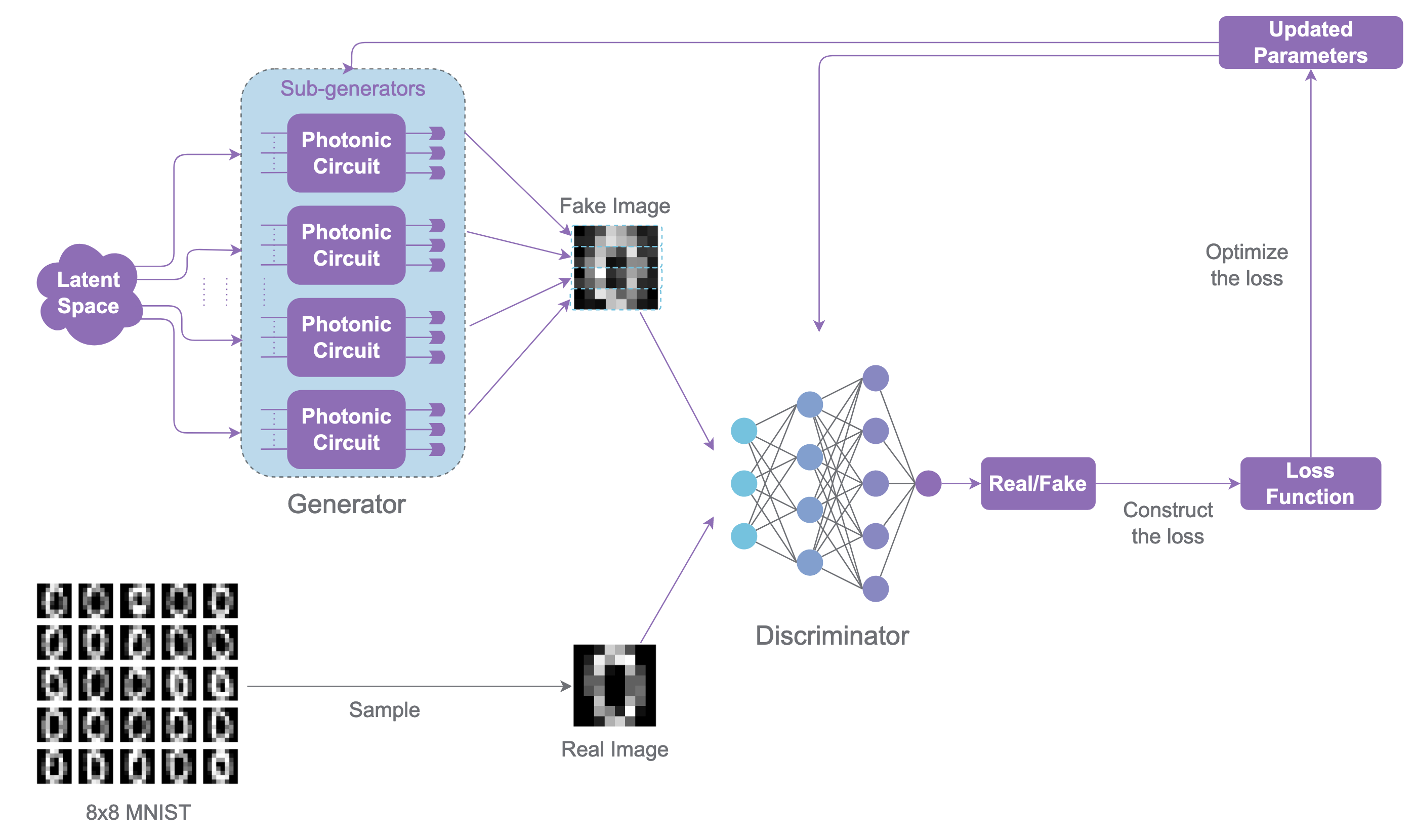
The model is composed of two different submodules: a generator G and a discriminator D which are competing against one another in an adversarial zero-sum game. The generator wants to fool the discriminator with fake images and the discriminator wants to correctly identify fake images versus real images from the dataset. The generator receives random noise values as input and transforms them to fake images of the dataset. The model can be identified in the next figure where we can just consider the generator as a whole classical model without the quantum sub generators.

The GAN has a specific training routine. Here are the main steps.

1. For a number of iterations:

   1. For a number of discriminator iterations d_steps:

      1. Train the discriminator parameters with the batches fake and real images. The labels of the real values are real_labels and the fake images’ labels are fake_labels. Here, after the hyper parameter optimization done in the reproduction, we will choose real_labels=0.9 and fake_labels=0.0.

   2. For a number of generator iterations g_steps:

      1. Train the generator parameters with only its fake generated images that have been classified by the discriminator. The associated labels are generator_labels. Here, after the hyper parameter optimization done in the reproduction, we will choose generator_labels=0.9.

The loss calculations for both steps are:

1. For the discriminator training

   \[\mathcal{L}_D=\frac{1}{n}\sum_{i=1}^n Loss(D(x_i),\text{real labels})+\frac{1}{n}\sum_{i=1}^n Loss(D(G(z_i)),\text{fake labels})\]

   where \(x_i\) is the real images of the batch and \(z_i\) are the noises generated for the batch.

2. For the generator training

   \[\mathcal{L}_G=\frac{1}{n}\sum_{i=1}^n Loss(D(G(z_i)),\text{generator labels})\]

   where \(z_i\) are the noises generated for the batch.

For the photonic QGAN, the preferred loss is PyTorch’s BCEWithLogitsLoss.

The photonic QGAN

The photonic implementation of the QGAN is similar. Just like it is illustrated in the picture, the generator will be composed of multiple photonic circuits that will be run together to generate brand new images. The concept and training of the GAN model stays the same.

from __future__ import annotations

import copy
import math
import random

import matplotlib.pyplot as plt
import numpy as np
import perceval as pcvl
import torch
from sklearn.datasets import load_digits
from torch import nn

import merlin as ML

Configuration

We will use the same experiment setup as the setup d of the reproduction. We will also use all of the optimized hyperparameters identified in the study of the photonic QGAN’s MerLin reproduction.

The demo uses four patch heads, two latent features, an 8 by 8 digit target (UCI Optdigits 0th digit), and one discriminator update followed by three generator updates. So, the dataset chosen here is 8x8 images of hand-drawn zeros.

seed = 0
digit = 0
training_iterations = 1400
batch_size = 4
image_size = 8
latent_dim = 2
generator_heads = 4

input_state = (0, 1, 0, 1, 0)

lr_d = 0.0002
lr_g = 0.004
adam_betas = (0.5, 0.99)
d_steps = 1
g_steps = 3

random.seed(seed)
np.random.seed(seed)
_ = torch.manual_seed(seed)

Load Optdigits Samples

The notebook uses sklearn.datasets.load_digits, so it can run without a separate data checkout. Pixel values are normalized to [0, 1].

digits = load_digits()
mask = digits.target == digit
real_images = torch.tensor(digits.images[mask], dtype=torch.float32).unsqueeze(1) / 16.0
real_vectors = real_images.reshape(real_images.shape[0], -1)

sample_generator = torch.Generator().manual_seed(seed + 17)
batch_indices = torch.randint(
    real_vectors.shape[0],
    (training_iterations, batch_size),
    generator=sample_generator,
)
real_batches = [real_vectors[indices] for indices in batch_indices]
real_preview = real_images[batch_indices[0]]

print(f"digit samples: {real_vectors.shape[0]}")
print(f"training batches: {len(real_batches)}")

digit samples: 178
training batches: 1400

Build the MerLin Photonic Generator

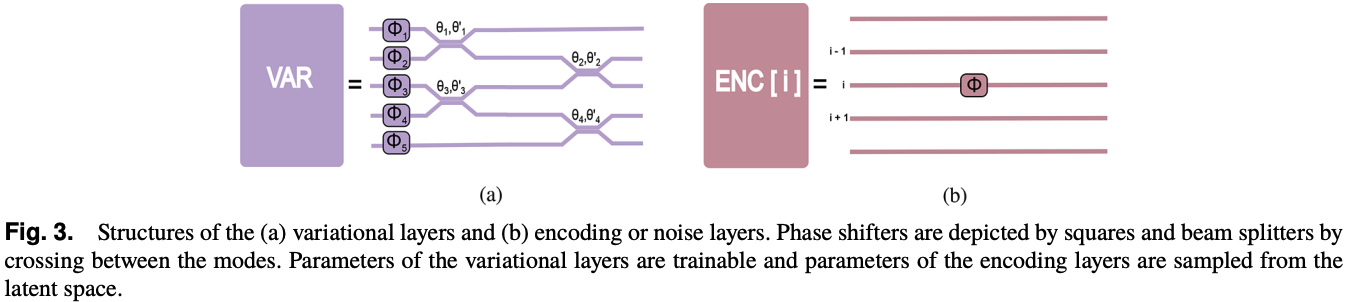
In order to get similar results as the one identified in the photonic QGAN paper and in the photonic QGAN reproduction with MerLin, we will use the same circuit unitaries as presented in the paper. Below is the photonic circuit implementation.

def var_circuit(n_modes: int, param_start_index: int = 0) -> pcvl.Circuit:
    """Create a trainable photonic circuit block for the generator.

    Parameters
    ----------
    n_modes : int
        Number of modes in the circuit.
    param_start_index : int
        Starting index for the trainable phase parameters.
        Default is 0.

    Returns
    -------
    pcvl.Circuit
        A Perceval circuit containing phase shifters and beam
        splitters with trainable parameters.
    """
    trainable_params = [pcvl.Parameter(f"phi{i+param_start_index}") for i in range((2 * n_modes) - 1)]
    circ = pcvl.Circuit(m=n_modes)
    for i in range(n_modes):
        circ.add([i], component=pcvl.PS(trainable_params[i]))
    for i, j in enumerate(range(0, n_modes - 1, 2)):
        circ.add([j, j + 1], component=pcvl.BS(trainable_params[i + n_modes]))
    for i, j in enumerate(range(1, n_modes - 1, 2)):
        circ.add([j, j + 1], component=pcvl.BS(trainable_params[i + n_modes + (n_modes // 2)]))

    return circ


def encoding_circuit(n_modes: int, mode_to_target: int, param_index: int = 0) -> pcvl.Circuit:
    """Create an encoding circuit that applies a phase to one mode.

    Parameters
    ----------
    n_modes : int
        Number of modes in the circuit.
    mode_to_target : int
        Mode index to apply the encoding phase shift.
    param_index : int
        Index for the encoding parameter.
        Default is 0.

    Returns
    -------
    pcvl.Circuit
        A Perceval circuit containing a single trainable phase shift.
    """
    encoding_param = pcvl.Parameter(f"theta{param_index}")
    circ = pcvl.Circuit(m=n_modes)
    circ.add([mode_to_target], component=pcvl.PS(encoding_param))

    return circ

We will then use those base bricks to create the subgenerator pattern d in the paper.

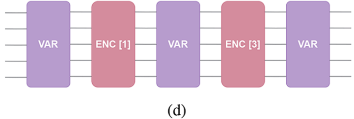
We will create a QuantumLayer out of these Perceval circuits created earlier.

In the original paper, the photonic generator can have or not photon-number-resolving detectors. Here, like on current Quandela hardware, we will suppose that the photon number cannot be resolved by the detectors.

def create_subgenerator(use_pnr_detectors:bool=False) -> ML.QuantumLayer:
    #Define the complete Perceval Circuit
    m=len(input_state)
    circuit=pcvl.Circuit(m=m)
    circuit.add(port_range=[i for i in range(m)],component=var_circuit(n_modes=m,param_start_index=0))
    circuit.add(port_range=[i for i in range(m)],component=encoding_circuit(n_modes=m,mode_to_target=1,param_index=0))
    circuit.add(port_range=[i for i in range(m)],component=var_circuit(n_modes=m,param_start_index=(2*m)-1))
    circuit.add(port_range=[i for i in range(m)],component=encoding_circuit(n_modes=m,mode_to_target=3,param_index=1))
    circuit.add(port_range=[i for i in range(m)],component=var_circuit(n_modes=m,param_start_index=(4*m)-2))

    #Define the Perceval experiment
    exp=pcvl.Experiment(circuit)

    #If the user does not want PNR detectors, remove them.
    if not use_pnr_detectors:
        for i in range(m):
            exp.detectors[i]=pcvl.Detector.threshold()

    #Create the corresponding QuantumLayer
    return ML.QuantumLayer(
        input_size=latent_dim,
        experiment=exp,
        input_state=input_state,
        trainable_parameters=["phi"],
        input_parameters=["theta"],
        measurement_strategy=ML.MeasurementStrategy.probs(
            computation_space=ML.ComputationSpace.FOCK,
            occupancy_readout=True,
        ),
    )

Let’s now define the PhotonicGenerator with this QuantumLayer.

We will use count=4 that creates four independent heads with the same circuit structure. Each head returns Fock-space probabilities with binary occupancy readout, then the image adapter maps each head to one patch of the generated image.

This is the same idea as presented in the paper to use multiple photonic circuits as patches to create one image.

generator = ML.PhotonicGenerator(
    layers=create_subgenerator(use_pnr_detectors=False),
    count=generator_heads,
    output_adapter=ML.ImageAdapter(
        shape=(1, image_size, image_size),
        headwise=True,
        normalize_patches=True,
    ),
)

fixed_noise = torch.normal(0.0, 2 * math.pi, (batch_size, latent_dim))
with torch.no_grad():
    generated_before = generator(fixed_noise).detach()

measurements = generator.measure(fixed_noise)
print(f"heads: {len(generator)}")
print(f"trainable parameters: {sum(p.numel() for p in generator.parameters())}")
print(f"per-head output widths: {[output.shape[1] for output in measurements.outputs]}")
print(f"image batch shape: {tuple(generated_before.shape)}")

heads: 4
trainable parameters: 108
per-head output widths: [15, 15, 15, 15]
image batch shape: (4, 1, 8, 8)

Defining the Classical Discriminator

The classical discriminator is just a regular pytorch module. We will use the same one as in the paper reproduction.

discriminator = nn.Sequential(
    nn.Linear(image_size * image_size, 32),
    nn.LeakyReLU(0.2),
    nn.Linear(32, 16),
    nn.LeakyReLU(0.2),
    nn.Linear(16, 1),
)

Train with Adam

In order to train the Photonic QGAN, we need to follow the specific training structure of the classical GAN. We will use the ADAM optimizer as it is the most fitted for MerLin use even though the original paper used SPSA. A study on the optimization of ADAM’s parameter is also available in the MerLin reproduction. It will be presented later. First, we need to define the performance metrics.

Defining the Metrics

We will use different metrics to analyze the training and performance of the photonic QGAN. We will define a batch similarity which determines how close the fake generated images of the current batch are close to the real images. This metric is basically the average of the structural similarity (ssim) over the full image (not exactly like skimage.metrics.structural_similarity) between all pairs of fake and real images on the batch.

def global_ssim(x: np.ndarray, y: np.ndarray) -> float:
    c1 = 0.01**2
    c2 = 0.03**2
    x = x.astype(np.float64, copy=False)
    y = y.astype(np.float64, copy=False)
    mu_x = float(x.mean())
    mu_y = float(y.mean())
    var_x = float(((x - mu_x) ** 2).mean())
    var_y = float(((y - mu_y) ** 2).mean())
    cov_xy = float(((x - mu_x) * (y - mu_y)).mean())
    numerator = (2 * mu_x * mu_y + c1) * (2 * cov_xy + c2)
    denominator = (mu_x**2 + mu_y**2 + c1) * (var_x + var_y + c2)
    return numerator / denominator


def batch_similarity(real: torch.Tensor, fake: torch.Tensor) -> float:
    real_batch = real.detach().cpu().numpy().reshape(batch_size, image_size, image_size)
    fake_batch = fake.detach().cpu().numpy().reshape(batch_size, image_size, image_size)
    total = 0.0
    for real_image in real_batch:
        for fake_image in fake_batch:
            total += global_ssim(
                np.clip(real_image, 0.0, 1.0),
                np.clip(fake_image, 0.0, 1.0),
            )
    return total / (batch_size * batch_size)

Training the Photonic QGAN

We will use the same training steps as the classical GAN to train our photonic QGAN. Since the generator and discriminator are ordinary PyTorch modules. loss.backward() populates gradients for the MerLin quantum layers, and the user-selected Adam optimizers own the parameter updates.

#Optimization objects
criterion = nn.BCEWithLogitsLoss()
optimizer_d = torch.optim.Adam(discriminator.parameters(), lr=lr_d, betas=adam_betas)
optimizer_g = torch.optim.Adam(generator.parameters(), lr=lr_g, betas=adam_betas)

#Generator's noise sampler
noise_generator = torch.Generator().manual_seed(seed + 31)

# Training results
d_losses: list[float] = []
g_losses: list[float] = []
similarity_scores: list[float] = []
best_similarity = float("-inf")
best_state = copy.deepcopy(generator.state_dict())
best_iteration = 0

#Labels used for the training
real_labels = torch.full((batch_size,), 0.9)
fake_labels = torch.zeros(batch_size)
generator_labels = torch.full((batch_size,), 0.9)


for iteration, real_data in enumerate(real_batches, start=1):

    # Discriminator training
    d_step_losses = []
    for _ in range(d_steps):
        noise_d = torch.normal(
            0.0,
            2 * math.pi,
            (batch_size, latent_dim),
            generator=noise_generator,
        )
        fake_for_d = generator(noise_d).reshape(batch_size, -1).detach()

        optimizer_d.zero_grad()
        d_loss = criterion(discriminator(real_data).view(-1), real_labels)
        d_loss = d_loss + criterion(discriminator(fake_for_d).view(-1), fake_labels)
        d_loss.backward()
        optimizer_d.step()
        d_step_losses.append(float(d_loss.detach()))


    # Freezing the discriminator for the generator training
    for parameter in discriminator.parameters():
        parameter.requires_grad_(False)

    # Generator training
    g_step_losses = []
    fake_for_metrics = None
    for _ in range(g_steps):
        noise_g = torch.normal(
            0.0,
            2 * math.pi,
            (batch_size, latent_dim),
            generator=noise_generator,
        )
        optimizer_g.zero_grad()
        fake_for_g = generator(noise_g).reshape(batch_size, -1)
        g_loss = criterion(discriminator(fake_for_g).view(-1), generator_labels)
        g_loss.backward()
        optimizer_g.step()
        g_step_losses.append(float(g_loss.detach()))
        fake_for_metrics = fake_for_g


    # Defreezing the discriminator for the discriminator training
    for parameter in discriminator.parameters():
        parameter.requires_grad_(True)

    if fake_for_metrics is None:
        raise RuntimeError("Generator update did not produce samples.")


    # Get the performance of the iteration
    similarity = batch_similarity(real_data, fake_for_metrics)
    if similarity > best_similarity:
        best_similarity = similarity
        best_iteration = iteration
        best_state = copy.deepcopy(generator.state_dict())

    d_losses.append(float(np.mean(d_step_losses)))
    g_losses.append(float(np.mean(g_step_losses)))
    similarity_scores.append(similarity)

#Checking the gradient
has_generator_gradient = any(
    parameter.grad is not None and parameter.grad.abs().sum() > 0
    for parameter in generator.parameters()
)

# Best result of the training
generator.load_state_dict(best_state)
with torch.no_grad():
    generated_best = generator(fixed_noise).detach()

print(f"training iterations: {training_iterations}")
print(f"best iteration: {best_iteration}")
print(f"best batch similarity: {best_similarity:.3f}")
print(f"generator gradients populated: {has_generator_gradient}")

training iterations: 1400
best iteration: 500
best batch similarity: 0.712
generator gradients populated: True

Results

The first row shows real digit-0 samples. The second row shows the generated digits before training. The third row shows the best checkpoint selected during the Adam run.

We then plot the losses and batch similarity scores per epoch.

def show_grid(images: torch.Tensor, title: str, axes: np.ndarray) -> None:
    flat_axes = axes.reshape(-1)
    for axis, image in zip(flat_axes, images, strict=False):
        axis.imshow(image.squeeze().cpu(), cmap="gray", vmin=0.0, vmax=1.0)
        axis.axis("off")
    for axis in flat_axes[len(images):]:
        axis.axis("off")
    axes[0].set_ylabel(title, rotation=0, labelpad=35, va="center")


fig, axes = plt.subplots(3, batch_size, figsize=(7, 4))
show_grid(real_preview, "real", axes[0])
show_grid(generated_before, "before", axes[1])
show_grid(generated_best, "best", axes[2])
fig.tight_layout()
plt.show()

fig, axes = plt.subplots(1, 2, figsize=(9, 3))
axes[0].plot(d_losses, label="D loss")
axes[0].plot(g_losses, label="G loss")
axes[0].set_xlabel("training iteration")
axes[0].set_ylabel("BCE loss")
axes[0].legend()

axes[1].plot(similarity_scores)
axes[1].axvline(best_iteration - 1, color="black", linestyle="--", linewidth=1)
axes[1].set_xlabel("training iteration")
axes[1].set_ylabel("batch similarity")
fig.tight_layout()
plt.show()

We observe the expected tendencies of the losses identified in the original paper. The generator loss increases as the discriminator ones decreases. Here, the best iteration is the 500th but the batch selection is chosen form 4 images: that means that this selection is dominated by batch noise. A more revealing metric would be to average it over multiple batches or iterations. The metric is a noisy per-batch proxy which is just to identify some good results.

What this demonstrates

This notebook exercises the public MerLin path needed by the photonic QGAN model: repeated independent generator heads via PhotonicGenerator(..., count=...), Fock-space occupancy readout, headwise image adaptation, a classical discriminator, and standard PyTorch Adam updates. The example is intentionally small; paper-scale experiments should use longer runs and checkpoint selection.