Neural Quantum Embedding: Pushing the Limits of Quantum Supervised Learning (nn_embedding)
This implementation is based on prior work by Hur et al..
The NQE model is composed of three submodels:
The classical model: Takes the input data and transforms it into the phases used by the the quantum embedder.
The quantum embedder: Encodes quantum states in respect to the output of the classical model.
The quantum classifier: Classifies the states generated by the quantum embedder.
The pipeline is separated into two phases.
Phase 1: The classical model is trained so that the quantum embedder generates states of different classes that are maximally distant.
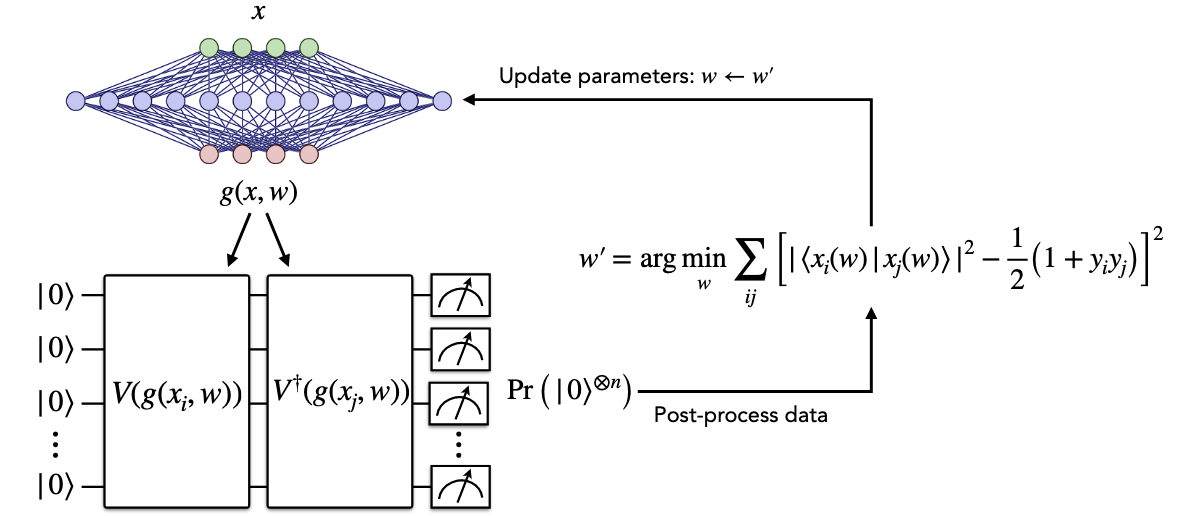
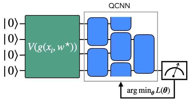
Phase 2: The quantum classifier is trained to classify the states generated by the classical model and quantum embedder.
This notebook will demonstrate the usage of a Neural Quantum Embedding as presented in the paper.
0. Setup and imports
[ ]:
import sys
import warnings
from pathlib import Path

import merlin as ml
import perceval as pcvl
import torch.nn as nn

REPO_ROOT = Path.cwd().resolve().parents[1]
sys.path.insert(0, str(REPO_ROOT))

warnings.filterwarnings("ignore")

from papers.nn_embedding.lib.merlin_based_model import (  # noqa: E402
    NeuralEmbeddingMerLinModel
)
from papers.nn_embedding.utils.data import (  # noqa: E402
    data_load_and_process
)
from papers.nn_embedding.utils.plotting import (  # noqa: E402
    plot_trace_distance,quick_loss_plot,plot_accuracies
)
1. Loading the Dataset To Classify (MNIST)
For the purpose of this tutorial, just like in the paper, we will classify the MNIST dataset restricted to the 0 and 1 digits. We will also apply PCA to this dataset to only have 8 features per image. We will use 300 samples per class.
[2]:
x_train, x_test, y_train, y_test = data_load_and_process(
            dataset="mnist",
            feature_reduction=8,
            classes=[0, 1],
            samples_per_class=300,
        )
y_test
[2]:
tensor([0, 0, 1, 1, 1, 1, 0, 1, 0, 1, 0, 0, 1, 1, 0, 1, 1, 1, 0, 1, 1, 0, 1, 1,
        1, 0, 0, 1, 0, 1, 0, 0, 0, 0, 0, 1, 0, 0, 1, 1, 0, 1, 1, 1, 1, 0, 1, 1,
        0, 1, 0, 1, 0, 0, 0, 0, 1, 0, 1, 0, 0, 1, 0, 1, 0, 0, 0, 1, 1, 1, 0, 0,
        1, 0, 0, 1, 0, 0, 1, 1, 0, 0, 0, 1, 1, 0, 1, 0, 0, 1, 1, 0, 0, 0, 0, 0,
        1, 1, 0, 0, 1, 1, 0, 1, 0, 1, 0, 1, 0, 1, 1, 1, 1, 1, 0, 1, 1, 0, 0, 1,
        1, 0, 1, 0, 0, 1, 1, 1, 1, 0, 1, 0, 0, 0, 0, 0, 1, 1, 1, 1, 0, 0, 1, 0,
        0, 0, 0, 0, 1, 1, 1, 1, 1, 1, 1, 0, 0, 1, 1, 1, 0, 0, 0, 0, 0, 1, 0, 1,
        1, 0, 0, 1, 0, 1, 1, 1, 1, 0, 0, 1, 0, 1, 0, 0, 1, 0, 0, 0, 1, 1, 1, 1,
        1, 0, 1, 0, 0, 1, 0, 0, 0, 1, 1, 0, 0, 1, 1, 0, 0, 1, 0, 0, 1, 0, 1, 0,
        0, 1, 0, 0, 0, 1, 1, 0, 0, 1, 0, 0, 1, 0, 1, 1, 1, 0, 0, 1, 0, 1, 1, 0,
        1, 1, 1, 0, 0, 1, 1, 1, 1, 1, 1, 1, 0, 0, 0, 0, 1, 0, 1, 1, 1, 0, 1, 1,
        0, 1, 0, 0, 1, 1, 1, 1, 1, 1, 1, 1, 1, 1, 1, 1, 1, 1, 1, 1, 0, 1, 0, 1,
        1, 1, 0, 0, 0, 0, 0, 0, 0, 0, 1, 0, 0, 0, 1, 1, 1, 0, 0, 0, 1, 1, 1, 1,
        0, 0, 1, 0, 1, 1, 1, 1, 1, 0, 1, 1, 1, 1, 1, 1, 1, 0, 1, 0, 0, 1, 0, 1,
        0, 1, 0, 0, 0, 0, 0, 0, 0, 1, 1, 1, 1, 0, 0, 1, 1, 1, 1, 0, 1, 0, 0, 0,
        1, 0, 1, 0, 0, 1, 0, 0, 0, 0, 0, 0, 0, 0, 0, 0, 0, 0, 0, 1, 0, 0, 1, 0,
        0, 0, 1, 0, 1, 0, 0, 1, 0, 0, 1, 1, 1, 1, 0, 0, 1, 0, 1, 0, 0, 0, 0, 0,
        0, 0, 1, 1, 0, 1, 1, 0, 1, 0, 1, 0, 0, 1, 0, 0, 1, 0, 0, 1, 1, 1, 1, 0,
        1, 1, 1, 1, 0, 1, 1, 1, 1, 0, 1, 0, 1, 0, 1, 1, 1, 0, 1, 0, 1, 1, 0, 1,
        1, 0, 0, 0, 1, 0, 0, 0, 0, 1, 1, 0, 1, 1, 0, 1, 0, 0, 0, 0, 0, 1, 1, 1,
        0, 0, 0, 0, 1, 1, 1, 0, 0, 0, 0, 1, 0, 1, 1, 1, 1, 1, 1, 1, 0, 1, 0, 1,
        0, 1, 1, 1, 1, 1, 1, 0, 1, 1, 1, 1, 1, 1, 1, 0, 0, 0, 1, 0, 0, 0, 0, 0,
        0, 1, 0, 0, 1, 1, 0, 0, 0, 0, 0, 1, 0, 1, 0, 0, 0, 0, 0, 1, 1, 0, 0, 1,
        0, 0, 1, 1, 0, 0, 1, 0, 1, 0, 0, 1, 0, 0, 0, 0, 0, 1, 1, 0, 0, 1, 0, 0,
        1, 1, 1, 0, 0, 0, 1, 0, 1, 0, 1, 1, 0, 1, 0, 0, 1, 0, 1, 1, 1, 1, 1, 1])
2. Create the models
In the nn_embedding pipeline, three models are needed.
An untrainable quantum embedder that takes for input the output of the classical model and prepares a state.
A trainable classical model that assigns parameters to the quantum embedder for a classical input.
A trainable quantum model that takes the encoded state and classifies the data.
Lets define these models.
2.1 Quantum embedder
This layer will receive its parameter values from the classical model. It encodes the features into quantum states via the classical model.
In this repository, for the MerLin based method, a universal unitary was given as the quantum embedder.
For MerLin models, the quantum embedder must be a MerLin QuantumLayer with input_size=0. The modifiable parameters will be the trainable ones that will be changed by the classical model. The embedder must not have amplitude encoding on and must return amplitudes.
[ ]:
circ = ml.CircuitBuilder(n_modes=8)
circ.add_entangling_layer()
embedder = ml.QuantumLayer(
    input_size=0,
    builder=circ,
    n_photons=4,
    measurement_strategy=ml.MeasurementStrategy.amplitudes(),
)
pcvl.pdisplay(circ.to_pcvl_circuit())
QuantumLayer(
  (_photon_loss_transform): PhotonLossTransform()
  (_detector_transform): DetectorTransform()
  (measurement_mapping): Amplitudes()
)
2.2 Classical model
This model will be trained to give the quantum embedder its optimal parameters for the classical input x.
Lets create a simple model with three linear layers. We need to match the last layer with the number of parameters in the quantum embedder.
[4]:
classical_model = nn.Sequential(
    nn.Linear(8, 10),
    nn.ReLU(),
    nn.Linear(10, 10),
    nn.ReLU(),
    nn.Linear(10,sum([i.numel() for i in embedder.parameters()])),
    )
classical_model
[4]:
Sequential(
  (0): Linear(in_features=8, out_features=10, bias=True)
  (1): ReLU()
  (2): Linear(in_features=10, out_features=10, bias=True)
  (3): ReLU()
  (4): Linear(in_features=10, out_features=56, bias=True)
)
2.3 Quantum classifier
This layer takes the encoded states and does the classification of the dataset.
We will once again use a universal unitary to train.
This model must be a QuantumLayer with amplitude encoding on and the probabilities measurement strategy.
[ ]:
circ = ml.CircuitBuilder(n_modes=8)
circ.add_entangling_layer()
classifier = ml.QuantumLayer(
    builder=circ,
    n_photons=4,
    measurement_strategy=ml.MeasurementStrategy.probs(),
)
pcvl.pdisplay(circ.to_pcvl_circuit())
QuantumLayer(
  (_photon_loss_transform): PhotonLossTransform()
  (_detector_transform): DetectorTransform()
  (measurement_mapping): Probabilities()
)
3. Create the main module
With those models created, we can combine them into the main module that executes the nn_embedding pipeline.
[6]:
model=NeuralEmbeddingMerLinModel(classical_model=classical_model,quantum_embedding_layer=embedder,quantum_classifier=classifier,num_classes=2)
model
[6]:
NeuralEmbeddingMerLinModel(
  (classical_encoder): Sequential(
    (0): Linear(in_features=8, out_features=10, bias=True)
    (1): ReLU()
    (2): Linear(in_features=10, out_features=10, bias=True)
    (3): ReLU()
    (4): Linear(in_features=10, out_features=56, bias=True)
  )
  (quantum_embedding_layer): QuantumLayer(
    (_photon_loss_transform): PhotonLossTransform()
    (_detector_transform): DetectorTransform()
    (measurement_mapping): Amplitudes()
  )
  (quantum_classifier): QuantumLayer(
    (_photon_loss_transform): PhotonLossTransform()
    (_detector_transform): DetectorTransform()
    (measurement_mapping): Probabilities()
  )
  (output_grouper): LexGrouping()
  (similarity_layer): _SimilarityLayer(
    (fidelity_layer): QuantumLayer(
      (_photon_loss_transform): PhotonLossTransform()
      (_detector_transform): DetectorTransform()
      (measurement_mapping): Probabilities()
    )
  )
  (embedding_training_model): _TrainingModule()
  (model): _TrainedEmbeddingModel(
    (quantum_classifier): QuantumLayer(
      (_photon_loss_transform): PhotonLossTransform()
      (_detector_transform): DetectorTransform()
      (measurement_mapping): Probabilities()
    )
  )
)
4. Train the embedding
The first part of the NQE pipeline is to train the embedding. To do so, you just need to call the train_embedding method of the object.
We will use the Adam optimiser with a 0.01 learning rate, the default optimizing procedure. We will also return the data which returns:
The loss per epoch
The trace distance between the average encoded state of each class for the train dataset.
The trace distance between the average encoded state of each class for the test dataset.
The loss lower bound generated by the encoded states of the training dataset.
The loss lower bound generated by the encoded states of the test dataset.
[7]:
losses_embedding,train_distances,test_distances,loss_lb_train,loss_lb_test=model.train_embedding(x_train=x_train,y_train=y_train,x_test=x_test,y_test=y_test,num_epochs=50,batch_size=150,return_data=True)
train_distances
Epoch 1 had a loss of 0.4416828453540802
Epoch 2 had a loss of 0.390857994556427
Epoch 3 had a loss of 0.3884666860103607
Epoch 4 had a loss of 0.28700536489486694
Epoch 5 had a loss of 0.24372565746307373
Epoch 6 had a loss of 0.1811673790216446
Epoch 7 had a loss of 0.12644872069358826
Epoch 8 had a loss of 0.09891556203365326
Epoch 9 had a loss of 0.07766833901405334
Epoch 10 had a loss of 0.0867651179432869
Epoch 11 had a loss of 0.0554957389831543
Epoch 12 had a loss of 0.04730817675590515
Epoch 13 had a loss of 0.05040502920746803
Epoch 14 had a loss of 0.04477526992559433
Epoch 15 had a loss of 0.03405756130814552
Epoch 16 had a loss of 0.027140477672219276
Epoch 17 had a loss of 0.037694141268730164
Epoch 18 had a loss of 0.04017558693885803
Epoch 19 had a loss of 0.04074986279010773
Epoch 20 had a loss of 0.0309336856007576
Epoch 21 had a loss of 0.021078528836369514
Epoch 22 had a loss of 0.04064815863966942
Epoch 23 had a loss of 0.04140010476112366
Epoch 24 had a loss of 0.01260322518646717
Epoch 25 had a loss of 0.01936456374824047
Epoch 26 had a loss of 0.020762905478477478
Epoch 27 had a loss of 0.01334301009774208
Epoch 28 had a loss of 0.020360765978693962
Epoch 29 had a loss of 0.020514748990535736
Epoch 30 had a loss of 0.01743766851723194
Epoch 31 had a loss of 0.012271538376808167
Epoch 32 had a loss of 0.015978697687387466
Epoch 33 had a loss of 0.013272665441036224
Epoch 34 had a loss of 0.014014815911650658
Epoch 35 had a loss of 0.011378418654203415
Epoch 36 had a loss of 0.005064515862613916
Epoch 37 had a loss of 0.015523694455623627
Epoch 38 had a loss of 0.007607364561408758
Epoch 39 had a loss of 0.015855232253670692
Epoch 40 had a loss of 0.013120574876666069
Epoch 41 had a loss of 0.014058787375688553
Epoch 42 had a loss of 0.020451905205845833
Epoch 43 had a loss of 0.011434332467615604
Epoch 44 had a loss of 0.007109335158020258
Epoch 45 had a loss of 0.004934689030051231
Epoch 46 had a loss of 0.014345008879899979
Epoch 47 had a loss of 0.003958116285502911
Epoch 48 had a loss of 0.013487202115356922
Epoch 49 had a loss of 0.0028921132907271385
Epoch 50 had a loss of 0.004696195479482412
[7]:
[tensor(0.2484),
 tensor(0.3307),
 tensor(0.4248),
 tensor(0.5226),
 tensor(0.6157),
 tensor(0.7027),
 tensor(0.7797),
 tensor(0.8397),
 tensor(0.8823),
 tensor(0.9081),
 tensor(0.9241),
 tensor(0.9325),
 tensor(0.9363),
 tensor(0.9343),
 tensor(0.9300),
 tensor(0.9231),
 tensor(0.9171),
 tensor(0.9114),
 tensor(0.9065),
 tensor(0.9035),
 tensor(0.9045),
 tensor(0.9086),
 tensor(0.9164),
 tensor(0.9254),
 tensor(0.9357),
 tensor(0.9435),
 tensor(0.9504),
 tensor(0.9567),
 tensor(0.9609),
 tensor(0.9629),
 tensor(0.9644),
 tensor(0.9659),
 tensor(0.9674),
 tensor(0.9688),
 tensor(0.9699),
 tensor(0.9706),
 tensor(0.9715),
 tensor(0.9726),
 tensor(0.9738),
 tensor(0.9747),
 tensor(0.9756),
 tensor(0.9763),
 tensor(0.9768),
 tensor(0.9772),
 tensor(0.9775),
 tensor(0.9775),
 tensor(0.9776),
 tensor(0.9776),
 tensor(0.9775),
 tensor(0.9774)]
5. Train the classifier
The second step of the nn_embedding pipeline is to train the quantum classifier. To do so, you just need to call the train_classifier method of the object.
We will use the Adam optimiser with a 0.01 learning rate, the default optimizing procedure. We will also return the data which returns:
The loss per epoch
The training accuracy per epoch
The test accuracy per epoch
[8]:
losses_classifier, train_accs, test_accs=model.train_classifier(x_train=x_train,y_train=y_train,x_test=x_test,y_test=y_test,batch_size=150,num_epochs=50,return_data=True)
test_accs
Epoch 1 had a loss of 0.5375056862831116
Epoch 2 had a loss of 0.5156368017196655
Epoch 3 had a loss of 0.5049517750740051
Epoch 4 had a loss of 0.486937016248703
Epoch 5 had a loss of 0.4807802736759186
Epoch 6 had a loss of 0.47028741240501404
Epoch 7 had a loss of 0.4555568993091583
Epoch 8 had a loss of 0.4455704689025879
Epoch 9 had a loss of 0.4213404953479767
Epoch 10 had a loss of 0.4204605519771576
Epoch 11 had a loss of 0.41078123450279236
Epoch 12 had a loss of 0.3885246813297272
Epoch 13 had a loss of 0.37565353512763977
Epoch 14 had a loss of 0.3763737380504608
Epoch 15 had a loss of 0.35390350222587585
Epoch 16 had a loss of 0.3487565517425537
Epoch 17 had a loss of 0.3409189283847809
Epoch 18 had a loss of 0.3226906955242157
Epoch 19 had a loss of 0.33411839604377747
Epoch 20 had a loss of 0.3156631290912628
Epoch 21 had a loss of 0.2979927659034729
Epoch 22 had a loss of 0.3003526031970978
Epoch 23 had a loss of 0.2885584533214569
Epoch 24 had a loss of 0.29112765192985535
Epoch 25 had a loss of 0.2562635540962219
Epoch 26 had a loss of 0.2651691138744354
Epoch 27 had a loss of 0.25815922021865845
Epoch 28 had a loss of 0.27444612979888916
Epoch 29 had a loss of 0.25244835019111633
Epoch 30 had a loss of 0.26817208528518677
Epoch 31 had a loss of 0.2758482098579407
Epoch 32 had a loss of 0.24227823317050934
Epoch 33 had a loss of 0.2306373119354248
Epoch 34 had a loss of 0.22668609023094177
Epoch 35 had a loss of 0.23772113025188446
Epoch 36 had a loss of 0.23967570066452026
Epoch 37 had a loss of 0.23423919081687927
Epoch 38 had a loss of 0.2541167140007019
Epoch 39 had a loss of 0.23082056641578674
Epoch 40 had a loss of 0.24062933027744293
Epoch 41 had a loss of 0.24220959842205048
Epoch 42 had a loss of 0.2155659794807434
Epoch 43 had a loss of 0.23781944811344147
Epoch 44 had a loss of 0.20480646193027496
Epoch 45 had a loss of 0.20538975298404694
Epoch 46 had a loss of 0.2209600806236267
Epoch 47 had a loss of 0.21725797653198242
Epoch 48 had a loss of 0.22399577498435974
Epoch 49 had a loss of 0.23558670282363892
Epoch 50 had a loss of 0.21998827159404755
[8]:
[42.833333333333336,
 50.166666666666664,
 51.333333333333336,
 54.333333333333336,
 60.0,
 67.0,
 76.16666666666667,
 80.83333333333333,
 84.66666666666667,
 85.83333333333333,
 88.16666666666667,
 89.5,
 90.16666666666667,
 90.33333333333333,
 90.83333333333333,
 91.16666666666667,
 91.33333333333333,
 91.33333333333333,
 91.5,
 91.66666666666667,
 91.83333333333333,
 91.83333333333333,
 92.66666666666667,
 93.83333333333333,
 94.16666666666667,
 94.66666666666667,
 94.83333333333333,
 95.33333333333333,
 95.83333333333333,
 96.5,
 96.66666666666667,
 97.0,
 97.83333333333333,
 98.33333333333333,
 98.5,
 98.5,
 98.5,
 98.5,
 98.5,
 98.66666666666667,
 98.83333333333333,
 99.0,
 99.16666666666667,
 99.16666666666667,
 99.16666666666667,
 99.16666666666667,
 99.33333333333333,
 99.33333333333333,
 99.33333333333333,
 99.33333333333333]
6. Plot the results
We will take the results and plot the training distance per embedding training epoch, the loss per classifier training epoch and the accuracies per classifier training epoch.
6.1. Trace distance plot
[9]:
plot_trace_distance(train_distances,test_distances,show=True)

<Figure size 640x480 with 0 Axes>
6.2. Loss plot
[10]:
quick_loss_plot(losses_classifier,show=True)

<Figure size 640x480 with 0 Axes>
6.3. Accuracy plot
[11]:
plot_accuracies(train_accs,test_accs,show=True)

<Figure size 640x480 with 0 Axes>
The same pipeline is used for the gate-based versions of this model (a few different technical details can be found in the docstrings of the objects). To reproduce the figure of the experiments, follow the steps in section 5 of the README.