Image classification with MerLin
This notebook presents three frameworks for image classification using MerLin and Perceval.
All of these frameworks are tested on the MNIST dataset to evaluate their effectiveness.
The three methods are:
Photonic QNN
A framework where a scale layer encodes the data into two trainable generic interferometers, complemented by a classifcation algorithm.
GLASE
A framework where a surrogate model simulates the gradients of a quantum layer, training a classical model to make predictions from this quantum layer.
Lancelot
A framework utilizing a custom gate to perform unitary dilation on the data, generating new features for prediction with a linear classifier.
All of these models originate from the GLASE repository on GitHub <https://github.com/Quandela/HybridAIQuantum-Challenge/blob/main/src/GLASE/model.py>_, created for the Perceval Quest challenge organized by Quandela.
First method, photonic qnn
I° Photonic QNN overview
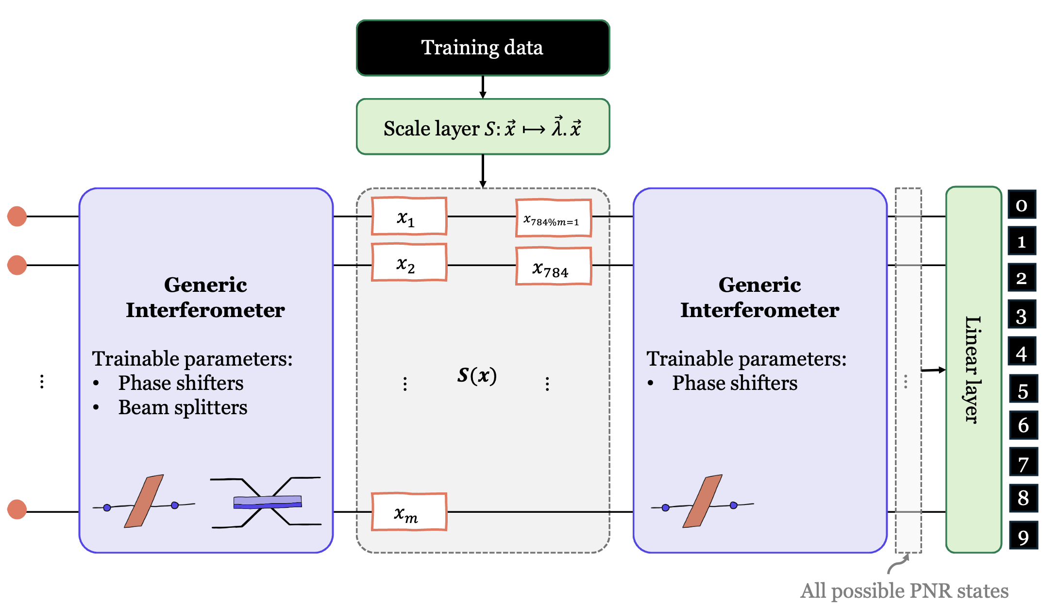 made by Vasileios Apostolou In this model, we initialise a first generic interferometer, fully trainable, then an encoding layer not trainable, and lastly an interferometer which only phase shifters are trainable.
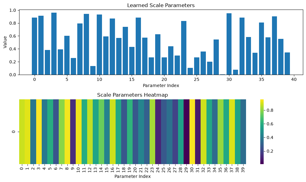
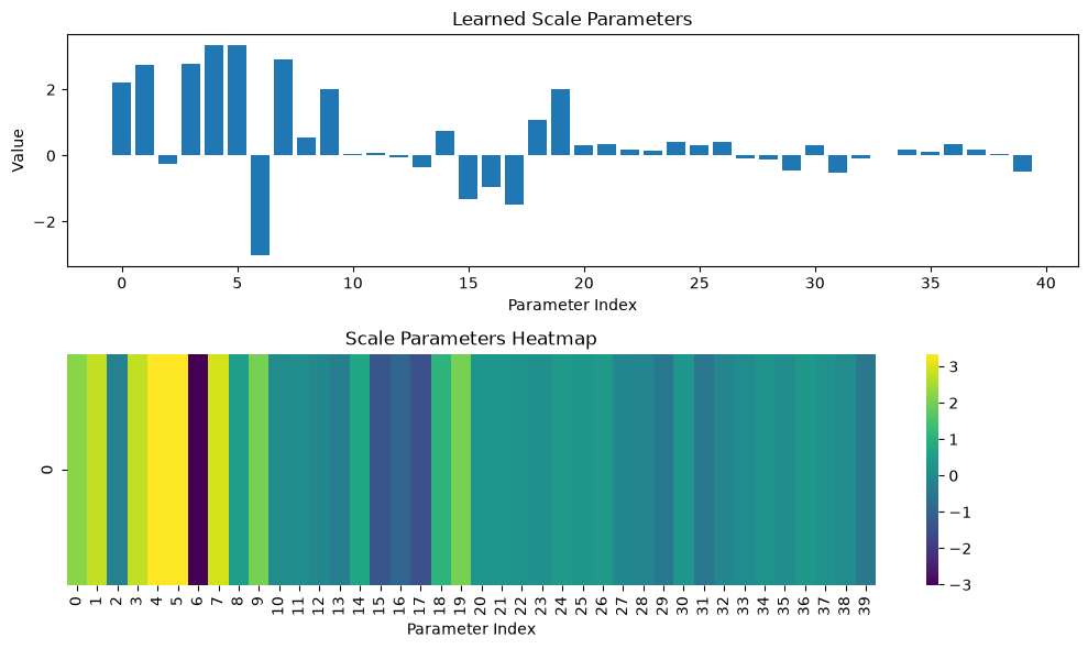
the trainable interferometer may need to rescale the input. that’s why we have to construct the ScaleLayer class.
[1]:
import math
import torch
import torch.nn as nn
import perceval as pcvl
from merlin.measurement.strategies import MeasurementStrategy
import os
import numpy as np
import pandas as pd
import matplotlib.pyplot as plt
import cma
from scipy import linalg
from tqdm.auto import tqdm
from sklearn.metrics import accuracy_score, confusion_matrix
import torch.optim as optim
from merlin import ComputationSpace, QuantumLayer, MeasurementStrategy, CircuitBuilder
import perceval.components as comp
import perceval.algorithm as algo
from perceval import catalog

import torch.nn.functional as F
from sklearn.metrics import confusion_matrix
from torch import nn
from torch.utils.data import Dataset, DataLoader, TensorDataset
from tqdm import tqdm
import random
import seaborn as sns
from sklearn.metrics import confusion_matrix, ConfusionMatrixDisplay
from sklearn.manifold import TSNE
import json
import re
from sklearn.preprocessing import StandardScaler, MinMaxScaler
from merlin.datasets import mnist_digits
from sklearn import svm
from sklearn.decomposition import PCA
from merlin.measurement import MeasurementStrategy
from collections.abc import Iterable
import pickle
from tqdm.auto import tqdm

from sklearn.preprocessing import MinMaxScaler
from torch.utils.data import DataLoader, TensorDataset

###############################
## Build the quantum circuit ##
###############################

INPUT_SIZE = 32

def create_quantum_circuit(m, size=40, frequency=1):
    """Create quantum circuit with specified number of modes"""
    # first trainable generic interferometer
    wl = pcvl.GenericInterferometer(m,
                                    lambda i: pcvl.BS(theta=pcvl.P(f"bs_1_{i}")) // pcvl.PS(pcvl.P(f"phase_1_{i}")) // \
                                              pcvl.BS(theta=pcvl.P(f"bs_2_{i}")) // pcvl.PS(pcvl.P(f"phase_2_{i}")),
                                    shape=pcvl.InterferometerShape.RECTANGLE)


    c = pcvl.Circuit(m)
    c.add(0, wl, merge=True)

    # f repetition of {encoding layers with input data in phase shifters; trainable generic interferometer}
    for f in range(frequency):
        c_var = pcvl.Circuit(m)
        for i in range(size):
            px = pcvl.P(f"px-{f}-{i + 1}")
            c_var.add(i % m, pcvl.PS(px))

        c.add(0, c_var, merge=True)

        wr = pcvl.GenericInterferometer(m,
                                        lambda i: pcvl.BS() // pcvl.PS(pcvl.P(f"phase_3_{i}")) // \
                                                  pcvl.BS() // pcvl.PS(pcvl.P(f"phase_4_{i}")),
                                        shape=pcvl.InterferometerShape.RECTANGLE)
        c.add(0, wr, merge=True)

    return c


class ScaleLayer(nn.Module):
    def __init__(self, dim, scale_type = "learned"):
        super(ScaleLayer, self).__init__()
        # Create a single learnable parameter (initialized to 1.0 by default)
        # Caution: MerLin already mutltiplies by pi
        if scale_type == "learned":
            self.scale = nn.Parameter(torch.rand(dim))
        elif scale_type == "2pi":
            self.scale = torch.full((dim,), 2)
        elif scale_type == "pi":
            self.scale = torch.full((dim,), 1)
        elif scale_type == "1":
            self.scale = torch.full((dim,), 1)
        #print(f"SELF.SCALE: {self.scale.shape}")

    def forward(self, x):
        # Element-wise multiplication of each input element by the learned scale
        return x * self.scale
/mnt/c/Users/LeïthKARRAÏ/PML-328/venvPML-250/lib/python3.12/site-packages/tqdm/auto.py:21: TqdmWarning: IProgress not found. Please update jupyter and ipywidgets. See https://ipywidgets.readthedocs.io/en/stable/user_install.html
  from .autonotebook import tqdm as notebook_tqdm
After the scale layer class construction, we can construct the core model, that we will use to make our classification. we will use perceval to make the circuit, and package it into merlin’s QuantumLayer class.
[2]:
class QLayer(nn.Module):
    def __init__(self, nb_photons, nb_modes, dim, scale_type="learned"):
        super().__init__()
        self.nb_modes = nb_modes
        self.nb_photons = nb_photons
        self.scaler = ScaleLayer(dim, scale_type)

        circuit = create_quantum_circuit(m=nb_modes, size=dim, frequency=1)

        input_state = [(i + 1) % 2 for i in range(nb_modes)]

        self.layer = QuantumLayer(
        input_size=dim,
        circuit=circuit,
        input_state=input_state,
        measurement_strategy=MeasurementStrategy.probs(),
        input_parameters=["px"],
        trainable_parameters=["bs", "phase"],
        )
    def forward(self, x):
        x = self.scaler(x)
        x = self.layer(x)

        return x
We can set the seed to reproduce the results.
[3]:
def set_seed(seed=42):
    """
    Set the random seed for reproducibility across different libraries.

    Args:
        seed (int): Seed value to use. Default is 42.
    """
    # Set Python's random seed
    random.seed(seed)

    # Set NumPy's random seed
    np.random.seed(seed)

    # Set PyTorch's random seeds for both CPU and CUDA
    torch.manual_seed(seed)
    if torch.cuda.is_available():
        torch.cuda.manual_seed(seed)
        torch.cuda.manual_seed_all(seed)  # For multi-GPU setups

    # Additional settings for complete reproducibility
    # Note: This can affect performance
    torch.backends.cudnn.deterministic = True
    torch.backends.cudnn.benchmark = False

    # For some PyTorch operations using Intel MKL
    os.environ['PYTHONHASHSEED'] = str(seed)

    print(f"Random seed set to {seed}")
II° and testing methods
first, we have to load the dataset and crop it to fit the model.
[4]:
class CustomToTensor:
    """
    Torch Tensor is not available with merlin 0.4, so we make a quick class to reliably replace toTensor method.

    """
    def __call__(self, pic):
        # Sécurité : forcer le type en numpy.ndarray si ce n'est pas déjà le cas
        if not isinstance(pic, np.ndarray):
            pic = np.array(pic)

        # 1. Réorganisation des dimensions si l'image a 3 dimensions (H, W, Canaux)
        if pic.ndim == 3:
            pic = pic.transpose((2, 0, 1))

        # 2. Conversion en tenseur PyTorch de type float
        img_tensor = torch.from_numpy(pic).float()

        # 3. Normalisation (seulement si l'image source était sur 8 bits)
        # Note : MNIST est souvent en uint8 [0, 255]
        if pic.dtype == np.uint8:
            img_tensor = img_tensor / 255.0

        return img_tensor


##########################
### load MNIST dataset ###
##########################

def crop_middle(image, size = 20):
    """
    Crop the middle from a numpy array based on the specified position.

    Args:
        image: Numpy array of shape (H, W, C) or (H, W)
        size: total size of the cropped image

    Returns:
        Cropped square numpy array
    """
    if len(image.shape) == 3:
        _, height, width = image.shape
    else:
        height, width = image.shape

    # Determine size of the square (the smaller dimension)
    mid_x = int(width * 0.5)
    mid_y = int(height * 0.5)
    half_size = int(size / 2)

    return image[mid_x-half_size:mid_x+half_size, mid_y-half_size:mid_y+half_size].copy()

class TransformCenter:
    def __init__(self, size = 20):
        self.transform = lambda x: crop_middle(x, size = size)
        self.tensor_transform = CustomToTensor()
        self.size = size

    def __call__(self, x):
        y1 = self.tensor_transform(self.transform(x)).view(self.size * self.size)
        return y1


# load the correct train, val dataset for the challenge, from the csv files
class MNIST_partial(Dataset):
    def __init__(self, data='./data', transform=None, split='train'):
        """
        Args:
            data: path to dataset folder which contains train.csv and val.csv
            transform (callable, optional): Optional transform to be applied
                on a sample (e.g., data augmentation or normalization)
            split: 'train' or 'val' to determine which set to download
        """
        self.data_dir = data
        self.transform = transform
        self.data = []

        if split == 'train':
            filename = os.path.join(self.data_dir, 'train.csv')
        elif split == 'val':
            filename = os.path.join(self.data_dir, 'val.csv')
        else:
            raise AttributeError("split!='train' and split!='val': split must be train or val")

        self.df = pd.read_csv(filename)

    def __len__(self):
        l = len(self.df['image'])
        return l

    def __getitem__(self, idx):
        img = self.df['image'].iloc[idx]
        label = self.df['label'].iloc[idx]
        # string to list
        img_list = re.split(r',', img)
        # remove '[' and ']'
        img_list[0] = img_list[0][1:]
        img_list[-1] = img_list[-1][:-1]
        # convert to float
        img_float = [float(el) for el in img_list]
        # convert to image
        img_square = torch.unflatten(torch.tensor(img_float), 0, (1, 28, 28)).numpy()
        #img_flat = img_square.flatten()
        if self.transform is not None:
            img_square = self.transform(img_square)
        return img_square, label


def load_dataset(size, bs):
    SIZE = size
    batch_size = bs

    # Load the Perceval Quest splits from the Merlin dataset helper
    X_train_raw, y_train_raw, _ = mnist_digits.get_data_train_percevalquest()
    X_val_raw, y_val_raw, _ = mnist_digits.get_data_test_percevalquest()

    # Crop a square at the centre of each image (SIZE x SIZE) and flatten it
    transform = TransformCenter(size=SIZE)
    X_train_flat = np.stack([transform(img).numpy() for img in X_train_raw]).astype(np.float32)
    X_val_flat = np.stack([transform(img).numpy() for img in X_val_raw]).astype(np.float32)

    y_train = np.asarray(y_train_raw, dtype=np.int64)
    y_val = np.asarray(y_val_raw, dtype=np.int64)

    # Feature-wise scaling (keeps behaviour identical to previous implementation)
    scaler = MinMaxScaler()
    X_train_scaled = scaler.fit_transform(X_train_flat)
    X_val_scaled = scaler.transform(X_val_flat)

    train_tensor = torch.from_numpy(X_train_scaled).float()
    val_tensor = torch.from_numpy(X_val_scaled).float()
    train_dataset = TensorDataset(train_tensor, torch.from_numpy(y_train))
    val_dataset = TensorDataset(val_tensor, torch.from_numpy(y_val))
    train_loader = DataLoader(train_dataset, batch_size=batch_size, shuffle=True)
    val_loader = DataLoader(val_dataset, batch_size=batch_size)

    INPUT_SIZE = SIZE * SIZE
    OUTPUT_FEATURES = 10

    return X_train_scaled, X_val_scaled, y_train, y_val, train_loader, val_loader, INPUT_SIZE, OUTPUT_FEATURES
III° training loop
we make the training loop for the photonic QNN
[5]:
def _classification_step(model, batch_X, batch_y, criterion, frequency):
    """Forward pass + loss for a plain classifier (photonic QNN or classical MLP).

    Returns the loss and a dict of predictions (single "measured" head).
    """
    batch_X = batch_X.repeat(1, 1, frequency)
    outputs = model(batch_X.squeeze(0).float())
    loss = criterion(outputs, batch_y)
    return loss, {"measured": outputs.argmax(dim=-1)}


def _hybrid_qnn_step(model, batch_X, batch_y, criterion, surrogate_rate):
    """Forward pass + loss for the CNN+QNN hybrid surrogate model.

    The model returns (out_approx, surrogate_loss, out_measured); the total loss
    blends the classical surrogate guidance, the surrogate-fidelity term, and the
    real quantum measurement. Returns the loss and a dict with both prediction heads.
    """
    out_approx, surrogate_loss, out_measured = model(batch_X)
    loss = (
        criterion(out_approx, batch_y) * 0.5
        + surrogate_loss * surrogate_rate
        + criterion(out_measured, batch_y) * 0.25
    )
    return loss, {"measured": out_measured.argmax(dim=-1), "approx": out_approx.argmax(dim=-1)}


def train_model(
    model,
    train_loader,
    val_loader,
    model_type="classification",
    num_epochs=25,
    lr=0.01,
    weight_decay=0.0,
    label_smoothing=0.0,
    frequency=1,
    device="cpu",
    save_path=None,
):
    """
    Unified training loop shared by the plain classifiers (photonic QNN / classical MLP)
    and the CNN+QNN hybrid surrogate model.

    Args:
        model: PyTorch model to train. For model_type="hybrid_qnn" it must return
            (out_approx, surrogate_loss, out_measured); otherwise it must return logits.
        train_loader: DataLoader for the training set.
        val_loader: DataLoader for the validation set.
        model_type (str): "classification" or "hybrid_qnn". Selects the forward/loss
            logic and the optimizer/scheduler configuration.
        num_epochs (int): number of training epochs.
        lr (float): learning rate.
        weight_decay (float): optimizer weight decay (only used for "hybrid_qnn").
        label_smoothing (float): label smoothing for CrossEntropyLoss.
        frequency (int): number of times the input is repeated for the encoding
            layer (only used for model_type="classification").
        device (str): device to train on.
        save_path (str | None): if provided, the model weights and history are
            pickled to this path (only meaningful for model_type="hybrid_qnn").

    Returns:
        history (dict): per-epoch train/val loss and accuracy (and surrogate
            accuracy, when model_type="hybrid_qnn").
        best_val_acc (float): best validation accuracy (%) reached, on the
            "measured" head.
    """
    model = model.to(device)
    criterion = nn.CrossEntropyLoss(label_smoothing=label_smoothing)
    step_fn = _hybrid_qnn_step if model_type == "hybrid_qnn" else _classification_step

    if model_type == "hybrid_qnn":
        optimizer = torch.optim.Adam(model.parameters(), lr=lr, weight_decay=weight_decay)
        scheduler = torch.optim.lr_scheduler.CosineAnnealingLR(optimizer, T_max=num_epochs, eta_min=2e-6)
    else:
        # Betas from the ablation study
        optimizer = torch.optim.Adam(model.parameters(), lr=lr, betas=(0.8, 0.999))
        scheduler = None

    surrogate_rate = 5.0
    history = {
        "train_loss": [], "val_loss": [],
        "train_acc": [], "val_acc": [],
        "train_acc_approx": [], "val_acc_approx": [],
    }
    best_val_acc = 0

    def run_epoch(loader, training, desc):
        model.train(training) if training else model.eval()
        total_loss, correct, correct_approx, total = 0.0, 0, 0, 0
        with torch.set_grad_enabled(training):
            for batch_X, batch_y in tqdm(loader, desc=desc, leave=False):
                batch_X, batch_y = batch_X.to(device), batch_y.to(device)
                if training:
                    optimizer.zero_grad()

                if model_type == "hybrid_qnn":
                    loss, preds = step_fn(model, batch_X, batch_y, criterion, surrogate_rate)
                else:
                    loss, preds = step_fn(model, batch_X, batch_y, criterion, frequency)

                if training:
                    loss.backward()
                    optimizer.step()

                total_loss += loss.item()
                total += batch_y.size(0)
                correct += (preds["measured"] == batch_y).sum().item()
                if "approx" in preds:
                    correct_approx += (preds["approx"] == batch_y).sum().item()

        avg_loss = total_loss / len(loader)
        acc = 100 * correct / total
        acc_approx = 100 * correct_approx / total if model_type == "hybrid_qnn" else acc
        return avg_loss, acc, acc_approx

    for epoch in range(num_epochs):
        train_loss, train_acc, train_acc_approx = run_epoch(
            train_loader, training=True, desc=f"Epoch {epoch + 1}/{num_epochs} [train]"
        )
        val_loss, val_acc, val_acc_approx = run_epoch(
            val_loader, training=False, desc=f"Epoch {epoch + 1}/{num_epochs} [val]"
        )

        best_val_acc = max(best_val_acc, val_acc)

        history["train_loss"].append(train_loss)
        history["val_loss"].append(val_loss)
        history["train_acc"].append(train_acc)
        history["val_acc"].append(val_acc)
        history["train_acc_approx"].append(train_acc_approx)
        history["val_acc_approx"].append(val_acc_approx)

        print(
            f"Epoch [{epoch + 1}/{num_epochs}], Train loss: {train_loss:.4f}, Val loss: {val_loss:.4f}, "
            f"Train acc: {train_acc:.4f}, Val acc: {val_acc:.4f}, Best val acc: {best_val_acc:.4f}"
        )

        if model_type == "hybrid_qnn":
            surrogate_rate *= 0.95
            scheduler.step()

    if save_path is not None:
        save_training_artifacts(model, history, model_type, save_path)

    return history, best_val_acc


# count paramaeters in a model (nn.Module)
def count_parameters(model):
    return sum(p.numel() for p in model.parameters() if p.requires_grad)
IV°/ Tests and results
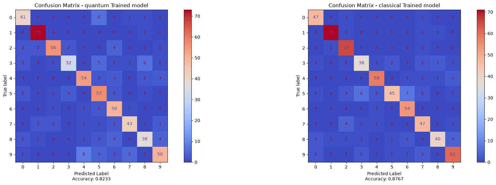
Once the training loop is done, we will be using confusion matrices to test the different models. tSNE will be used to show the results of the model, by extracting features via extract_features function, and ploting it withdisplay_tsne. tsne is an algorithm of non-supervised learning which perform classification, if the model perform well, tsne will be really efficient. we will also visualize the scale parameters of the encoding function and then save the results.
[6]:
#############################
### results visualisation ###
#############################
## here, we want to visualize the scale parameters of the encoding function ##
def visualize_scale_parameters(scale_layer):
    """
        Display scale parameters of the encoding layers.

        Args:
            scale_layer (nn.Module): encoding layer
        """
    # Get the scale parameter data as a numpy array
    scale_data = scale_layer.scale.data.cpu().numpy()

    # For a single scale parameter
    if scale_data.size == 1:
        print(f"Learned scale parameter: {scale_data.item():.4f}")

    # For a 1D array of parameters (e.g., per feature)
    elif len(scale_data.shape) == 1 or (
            len(scale_data.shape) > 1 and np.prod(scale_data.shape) == max(scale_data.shape)):
        # Reshape to 1D if necessary
        scale_data = scale_data.flatten()

        plt.figure(figsize=(10, 6))

        # Option 1: Bar plot
        plt.subplot(2, 1, 1)
        plt.bar(range(len(scale_data)), scale_data)
        plt.title('Learned Scale Parameters')
        plt.xlabel('Parameter Index')
        plt.ylabel('Value')

        # Option 2: Heatmap (1D version)
        plt.subplot(2, 1, 2)
        sns.heatmap(scale_data.reshape(1, -1), cmap='viridis', annot=True if len(scale_data) < 20 else False)
        plt.title('Scale Parameters Heatmap')
        plt.xlabel('Parameter Index')

        plt.tight_layout()
        plt.savefig('scale_parameters.png')
        plt.show()

## display the confusion matrices for the 2 models ##
def display_confusion_matrices(model1, model2, val_loader, class_names=None, device='cuda'):
    """
    Display confusion matrices for two trained models using a validation data loader.

    Args:
        3 models : 3 PyTorch model
        val_loader: PyTorch DataLoader containing validation data
        class_names: List of class names (optional)
        device: Device to run inference on ('cuda' or 'cpu')
    """
    # Set models to evaluation mode
    model1.eval()
    model2.eval()

    # Move models to the appropriate device
    model1 = model1.to(device)
    model2 = model2.to(device)

    # Initialize lists to store predictions and ground truth
    all_preds1 = []
    all_preds2 = []
    all_targets = []

    # Disable gradient computation for inference
    with torch.no_grad():
        for inputs, targets in val_loader:

            targets = targets.to(device)

            # Get predictions from both models
            # outputs1 = model1(inputs.squeeze(1).float())
            # outputs2 = model2(inputs.squeeze(1).float())
            outputs1 = model1((inputs.squeeze(1).float()))
            outputs2 = model2((inputs.squeeze(1).float()))

            # Convert outputs to class predictions
            _, preds1 = torch.max(outputs1, 1)
            _, preds2 = torch.max(outputs2, 1)

            # Append batch predictions and targets to lists
            all_preds1.extend(preds1.cpu().numpy())
            all_preds2.extend(preds2.cpu().numpy())
            all_targets.extend(targets.cpu().numpy())

    # Convert lists to numpy arrays
    all_preds1 = np.array(all_preds1)
    all_preds2 = np.array(all_preds2)
    all_targets = np.array(all_targets)

    # Compute confusion matrices
    cm1 = confusion_matrix(all_targets, all_preds1)
    cm2 = confusion_matrix(all_targets, all_preds2)

    # Create a figure with two subplots
    fig, (ax1, ax2) = plt.subplots(1, 2, figsize=(20, 6))

    # Display confusion matrices
    disp1 = ConfusionMatrixDisplay(confusion_matrix=cm1, display_labels=class_names)
    disp2 = ConfusionMatrixDisplay(confusion_matrix=cm2, display_labels=class_names)

    disp1.plot(ax=ax1, cmap='coolwarm', values_format='d')
    disp2.plot(ax=ax2, cmap='coolwarm', values_format='d')

    # Set titles
    ax1.set_title('Confusion Matrix - quantum Trained model')
    ax2.set_title('Confusion Matrix - classical Trained model')

    # Add overall accuracy to the titles
    acc1 = np.sum(np.diag(cm1)) / np.sum(cm1)
    acc2 = np.sum(np.diag(cm2)) / np.sum(cm2)

    ax1.set_xlabel(f'Predicted Label\nAccuracy: {acc1:.4f}')
    ax2.set_xlabel(f'Predicted Label\nAccuracy: {acc2:.4f}')

    plt.tight_layout()
    #plt.savefig(f'./results/CM-h-{hidden_dim}-m-{modes}.png')
    plt.show()

    return cm1, cm2

## extract features from a trained model for tSNE analysis ##
def extract_features(model, dataloader, device='cuda'):
    """
        Extract features using a trained model.

        Args:
            models : PyTorch model from which to extract features
            dataloader: dataloader containing training/validation data
            device: Device to run inference on ('cuda' or 'cpu')

        Returns:
            features: TorchTensor
            labels: TorchTensor
    """
    model.eval()  # Set the model to evaluation mode
    features = []
    labels = []

    with torch.no_grad():
        for data, label in dataloader:
            BS = data.shape[0]
            data = data.reshape(BS,-1).to(device)
            #print(f"\nData = {data}")
            output = model(data.float())
            features.append(output.cpu())  # Move to CPU for compatibility
            labels.extend(label.cpu().numpy())

    features = torch.cat(features, dim=0).numpy()
    labels = torch.tensor(labels).numpy()
    return features, labels


## display the tSNE plots for 2 models and dataloader ##
def display_tsne(model1, model2, val_loader,modes, device='cpu'):
    """
    Display the 3 tSNE for 3 trained models using a validation data loader.

    Args:
        the 2 models: 2 PyTorch models we want to compare
        val_loader: PyTorch DataLoader containing validation data
        modes: number used for the quantum model (for the Figure title)
        device: Device to run inference on ('cuda' or 'cpu')
    """
    # Set models to evaluation mode
    model1.eval()
    model2.eval()

    # Move models to the appropriate device
    model1 = model1.to(device)
    model2 = model2.to(device)

    # get the features and compute tSNE for each model
    features_1, labels_1 = extract_features(model1, val_loader, device=device)
    tsne = TSNE(n_components=2, random_state=42)
    features_2d_1 = tsne.fit_transform(features_1)

    features_2, labels_2 = extract_features(model2, val_loader, device=device)
    tsne = TSNE(n_components=2, random_state=42)
    features_2d_2 = tsne.fit_transform(features_2)


    # Display the tSNE plots
    fig, (ax1, ax2) = plt.subplots(1, 2, figsize=(20, 5))
    num_classes = 10
    for class_idx in range(num_classes):
        ax1.scatter(features_2d_1[labels_1 == class_idx, 0], features_2d_1[labels_1 == class_idx, 1],
                    label=f'Digit {class_idx}', alpha=0.6)
        ax1.set_xlabel('t-SNE Dim 1')
        ax1.set_ylabel('t-SNE Dim 2')
        ax1.legend()
        ax2.scatter(features_2d_2[labels_2 == class_idx, 0], features_2d_2[labels_2 == class_idx, 1],
                    label=f'Digit {class_idx}', alpha=0.6)
        ax2.set_xlabel('t-SNE Dim 1')
        ax2.set_ylabel('t-SNE Dim 2')
        ax2.legend()

    # Set titles
    ax1.set_title('tSNE - quantum kernel')
    ax2.set_title('tSNE - classical kernel model')
    plt.tight_layout()
    plt.savefig(f'tSNE-m-{modes}.png')
    #plt.show()

    return "done"

def save_experiment_results(results, filename='photonic_qNN_results.json'):
    """
    Append experiment results to a JSON file.

    Args:
        results (dict): Dictionary containing experiment results (with float values)
        filename (str): Path to the JSON file to store results
    """
    # Check if file exists and load existing data
    if os.path.exists(filename):
        try:
            with open(filename, 'r') as file:
                all_results = json.load(file)
        except json.JSONDecodeError:
            # Handle case where file exists but is empty or corrupted
            all_results = []
    else:
        all_results = []

    # Append new results
    all_results.append(results)

    # Write updated data back to file
    with open(filename, 'w') as file:
        json.dump(all_results, file, indent=4)

    return len(all_results)
V°/ Main loop
the different training paramaters are : batch_size : size of the batches. size : the size of the encoding layer. pca_comp : The number of components resulting from pca. pca_enabled : boolean to enable pca display : boolean to display number of paramters, the results. FREQUENCY : number ofphase shifters in the encoding layer. MODES : number of modes. epochs: number of epochs. lr : learning rate. At first, we load the datasets and reduce the paramaters (if pca
enabled), then we initiate the quantum layer and show the parameters. We also initiate a classical model and an svm to compare with the model. we lauch the training loop, plot and save the results.
[7]:
def main():
    set_seed(42)

    batch_size = 64
    size = 28
    pca_comp = 40
    pca_enabled = True
    display = True
    FREQUENCY = 1
    MODES = 10
    epochs = 32
    lr = 0.05


    # load data
    print("\n Loading dataset...")
    X_train,X_val,y_train,y_val, train_loader,val_loader, INPUT_SIZE, OUTPUT_FEATURES = load_dataset(size, batch_size)
    print(f"... data loader with input size = {INPUT_SIZE}")
    print(f" - training statistics: \n - X_train: {X_train.shape} \n - X_val: {X_val.shape}")

    # Reduce to desired number of components (e.g., 40)
    if pca_enabled:
        print("\n - Extracting PCA components")
        n_components = pca_comp
        pca = PCA(n_components=n_components)

        X_pca = pca.fit_transform(X_train.reshape(X_train.shape[0], size*size))
        X_val_pca = pca.transform(X_val.reshape(X_val.shape[0], size*size))

        X_pca = torch.sigmoid(torch.FloatTensor(X_pca))
        X_val_pca = torch.sigmoid(torch.FloatTensor(X_val_pca))
        print(X_pca.shape)
        print(X_pca[2])

        train_dataset = TensorDataset(X_pca, torch.LongTensor(y_train))
        train_loader = DataLoader(train_dataset, batch_size=batch_size, shuffle=True)
        val_dataset = TensorDataset(X_val_pca, torch.LongTensor(y_val))
        val_loader = DataLoader(val_dataset, batch_size=batch_size)
        INPUT_SIZE = n_components

    ##################
    ## photonic qNN ##
    ##################
    print("\n - Building the photonic quantum neural network...")
    input_state = [(i + 1) % 2 for i in range(MODES)]
    photons_count = sum(input_state)
    print(f"input state: {input_state}")

    Q_Layer = QLayer(photons_count, MODES, INPUT_SIZE*FREQUENCY, scale_type="learned")


    # learnable layer to map to the correct number of classes
    #classification_layer = nn.Linear(in_features=math.comb(MODES + photons_count-1,photons_count), out_features=OUTPUT_FEATURES,
    #                                 bias=True)
    classification_layer = nn.Linear(in_features=math.comb(MODES, photons_count), out_features=OUTPUT_FEATURES, bias=True)
    # input layer that multiplies the input by a learned encoding
    # input_layer = ScaleLayer(INPUT_SIZE*FREQUENCY, scale_type="learned")

   # Q_Layer = QLayer(photons_count, MODES, size*FREQUENCY, scale_type="learned")
    if display:
        visualize_scale_parameters(Q_Layer.scaler)
    #nn.init.xavier_uniform_(classification_layer.weight)
    #nn.init.constant_(classification_layer.bias, 0.0)
    # create q_model as nn.Module
    q_model = nn.Sequential(Q_Layer, classification_layer)
    print("... Model built")

    ########################
    ## classical NN (MLP) ##
    ########################
    # 2 layers with ReLU activation
    layer_1 = nn.Linear(in_features=INPUT_SIZE, out_features=32, bias=True)
    layer_2 = nn.Linear(in_features=32, out_features=OUTPUT_FEATURES, bias=True)
    model = nn.Sequential(layer_1, nn.ReLU(), layer_2, nn.Softmax(dim=1))

    #########################
    ## Training the models ##
    #########################

    EPOCHS = epochs
    LR = lr

    print(f" --- Training the quantum NN")

    q_history, best_q_acc = train_model(
        q_model, train_loader, val_loader,
        model_type="classification", num_epochs=EPOCHS, lr=LR, frequency=FREQUENCY,
    )
    q_train_losses, q_val_losses = q_history["train_loss"], q_history["val_loss"]
    q_train_accs, q_val_accs = q_history["train_acc"], q_history["val_acc"]
    if display:
        visualize_scale_parameters(q_model[0].scaler)
        # save qLayer if needed
        #torch.save(q_model[0].state_dict(), 'scale_layer_trained_5.pt')

    # train classical baseline
    print(f" --- Training the classical NN (linear)")
    cl_history, best_cl_acc = train_model(
        model, train_loader, val_loader,
        model_type="classification", num_epochs=EPOCHS, lr=0.01,
    )
    cl_train_losses, cl_val_losses = cl_history["train_loss"], cl_history["val_loss"]
    cl_train_accs, cl_val_accs = cl_history["train_acc"], cl_history["val_acc"]

    ### APPLY SVM ###
    print("--- APPLYING a SVM ---")
    clf = svm.SVC()
    clf.fit(X_train, y_train)
    svm_acc = clf.score(X_val, y_val)
    print(f" -> Validation Accuracy after SVM: {svm_acc}")
    print("--- SVM applied ---")

    print(f" - TRAINING IS DONE - \n - Best validation accuracy for the quantum kernel = {best_q_acc:.4f} (for {count_parameters(q_model)} parameters),"
          f" \n - Best validation accuracy for the linear kernel = {best_cl_acc:.4f} (for {count_parameters(model)} parameters)")

    # display tSNE and confusion matrices if asked in arguments
    if display:
        print("\n - Computing the confusion matrices...")
        display_confusion_matrices(q_model, model, val_loader, device = 'cpu')
        print(" - Computing the tSNE plots")
        display_tsne(nn.Sequential(q_model[0], q_model[1]), model[0], val_loader, MODES, device="cpu")

    # save results
    print("\n - Saving results...")
    result_dict = {"dataset": "mnist",
            "learnable scale": True ,
            "best q ACC": best_q_acc, "best cl ACC": best_cl_acc,
            "q parameters":count_parameters(q_model),"cl parameters":count_parameters(model)}
    save_experiment_results(result_dict)
    print("Results saved !")
    print("\nEXPERIMENT COMPLETE !")


if __name__ == "__main__":
    main()
Random seed set to 42

 Loading dataset...
/tmp/ipykernel_39283/1849384163.py:132: UserWarning: The given NumPy array is not writable, and PyTorch does not support non-writable tensors. This means writing to this tensor will result in undefined behavior. You may want to copy the array to protect its data or make it writable before converting it to a tensor. This type of warning will be suppressed for the rest of this program. (Triggered internally at /pytorch/torch/csrc/utils/tensor_numpy.cpp:213.)
  train_dataset = TensorDataset(train_tensor, torch.from_numpy(y_train))
... data loader with input size = 784
 - training statistics:
 - X_train: (6000, 784)
 - X_val: (600, 784)

 - Extracting PCA components
torch.Size([6000, 40])
tensor([0.4309, 0.8457, 0.6219, 0.1639, 0.8497, 0.3872, 0.2632, 0.8520, 0.4542,
        0.3130, 0.6797, 0.7341, 0.1836, 0.8542, 0.2123, 0.2716, 0.6835, 0.5003,
        0.5657, 0.8262, 0.7604, 0.4670, 0.3492, 0.5485, 0.5509, 0.6220, 0.3030,
        0.7560, 0.7189, 0.3557, 0.3678, 0.6472, 0.5085, 0.2901, 0.6294, 0.3622,
        0.8265, 0.2789, 0.6888, 0.3700])

 - Building the photonic quantum neural network...
input state: [1, 0, 1, 0, 1, 0, 1, 0, 1, 0]
... Model built
 --- Training the quantum NN
Epoch [1/32], Train loss: 1.7820, Val loss: 1.4260, Train acc: 38.9833, Val acc: 49.5000, Best val acc: 49.5000
Epoch [2/32], Train loss: 1.2675, Val loss: 1.1422, Train acc: 56.4000, Val acc: 60.3333, Best val acc: 60.3333
Epoch [3/32], Train loss: 1.1038, Val loss: 1.0305, Train acc: 61.6167, Val acc: 65.8333, Best val acc: 65.8333
Epoch [4/32], Train loss: 0.9052, Val loss: 0.8361, Train acc: 69.2333, Val acc: 71.5000, Best val acc: 71.5000
Epoch [5/32], Train loss: 0.8297, Val loss: 0.9117, Train acc: 72.3500, Val acc: 67.0000, Best val acc: 71.5000
Epoch [6/32], Train loss: 0.8377, Val loss: 0.7386, Train acc: 72.3000, Val acc: 76.1667, Best val acc: 76.1667
Epoch [7/32], Train loss: 0.7713, Val loss: 0.7762, Train acc: 74.7333, Val acc: 73.1667, Best val acc: 76.1667
Epoch [8/32], Train loss: 0.7347, Val loss: 0.7471, Train acc: 75.7000, Val acc: 76.5000, Best val acc: 76.5000
Epoch [9/32], Train loss: 0.7196, Val loss: 0.7100, Train acc: 76.2833, Val acc: 75.5000, Best val acc: 76.5000
Epoch [10/32], Train loss: 0.7016, Val loss: 0.8323, Train acc: 76.9167, Val acc: 71.0000, Best val acc: 76.5000
Epoch [11/32], Train loss: 0.7430, Val loss: 0.7396, Train acc: 75.1333, Val acc: 74.5000, Best val acc: 76.5000
Epoch [12/32], Train loss: 0.6947, Val loss: 0.7405, Train acc: 76.0500, Val acc: 73.0000, Best val acc: 76.5000
Epoch [13/32], Train loss: 0.6873, Val loss: 0.7214, Train acc: 77.1833, Val acc: 75.8333, Best val acc: 76.5000
Epoch [14/32], Train loss: 0.6874, Val loss: 0.7932, Train acc: 76.9333, Val acc: 74.0000, Best val acc: 76.5000
Epoch [15/32], Train loss: 0.6651, Val loss: 0.6072, Train acc: 78.3333, Val acc: 78.6667, Best val acc: 78.6667
Epoch [16/32], Train loss: 0.6689, Val loss: 0.6957, Train acc: 77.4167, Val acc: 76.1667, Best val acc: 78.6667
Epoch [17/32], Train loss: 0.6489, Val loss: 0.6114, Train acc: 78.2500, Val acc: 81.0000, Best val acc: 81.0000
Epoch [18/32], Train loss: 0.6649, Val loss: 0.7060, Train acc: 77.3500, Val acc: 76.5000, Best val acc: 81.0000
Epoch [19/32], Train loss: 0.6312, Val loss: 0.6078, Train acc: 78.6500, Val acc: 78.6667, Best val acc: 81.0000
Epoch [20/32], Train loss: 0.6225, Val loss: 0.6076, Train acc: 79.1667, Val acc: 80.0000, Best val acc: 81.0000
Epoch [21/32], Train loss: 0.6316, Val loss: 0.5470, Train acc: 79.2833, Val acc: 81.8333, Best val acc: 81.8333
Epoch [22/32], Train loss: 0.6009, Val loss: 0.6109, Train acc: 80.2667, Val acc: 80.0000, Best val acc: 81.8333
Epoch [23/32], Train loss: 0.6201, Val loss: 0.6658, Train acc: 79.7833, Val acc: 77.8333, Best val acc: 81.8333
Epoch [24/32], Train loss: 0.6140, Val loss: 0.6240, Train acc: 79.7500, Val acc: 78.5000, Best val acc: 81.8333
Epoch [25/32], Train loss: 0.5992, Val loss: 0.6894, Train acc: 80.1333, Val acc: 75.3333, Best val acc: 81.8333
Epoch [26/32], Train loss: 0.5923, Val loss: 0.5962, Train acc: 80.4667, Val acc: 79.6667, Best val acc: 81.8333
Epoch [27/32], Train loss: 0.5923, Val loss: 0.5469, Train acc: 80.2667, Val acc: 83.3333, Best val acc: 83.3333
Epoch [28/32], Train loss: 0.5716, Val loss: 0.5986, Train acc: 81.2333, Val acc: 82.1667, Best val acc: 83.3333
Epoch [29/32], Train loss: 0.5911, Val loss: 0.5939, Train acc: 80.4167, Val acc: 78.8333, Best val acc: 83.3333
Epoch [30/32], Train loss: 0.5991, Val loss: 0.6353, Train acc: 79.9667, Val acc: 78.8333, Best val acc: 83.3333
Epoch [31/32], Train loss: 0.5723, Val loss: 0.5881, Train acc: 81.2833, Val acc: 82.0000, Best val acc: 83.3333
Epoch [32/32], Train loss: 0.5751, Val loss: 0.5676, Train acc: 81.1000, Val acc: 82.3333, Best val acc: 83.3333
--- Training the classical NN (linear)
Epoch [1/32], Train loss: 2.1441, Val loss: 1.9530, Train acc: 36.8167, Val acc: 56.6667, Best val acc: 56.6667
Epoch [2/32], Train loss: 1.8422, Val loss: 1.7856, Train acc: 68.0500, Val acc: 70.5000, Best val acc: 70.5000
Epoch [3/32], Train loss: 1.7404, Val loss: 1.7030, Train acc: 76.5000, Val acc: 80.8333, Best val acc: 80.8333
Epoch [4/32], Train loss: 1.6734, Val loss: 1.6590, Train acc: 83.7167, Val acc: 84.1667, Best val acc: 84.1667
Epoch [5/32], Train loss: 1.6336, Val loss: 1.6223, Train acc: 86.4500, Val acc: 87.1667, Best val acc: 87.1667
Epoch [6/32], Train loss: 1.6174, Val loss: 1.6153, Train acc: 86.8000, Val acc: 87.8333, Best val acc: 87.8333
Epoch [7/32], Train loss: 1.6046, Val loss: 1.6120, Train acc: 87.7000, Val acc: 87.3333, Best val acc: 87.8333
Epoch [8/32], Train loss: 1.5982, Val loss: 1.6028, Train acc: 88.0333, Val acc: 87.5000, Best val acc: 87.8333
Epoch [9/32], Train loss: 1.5938, Val loss: 1.6298, Train acc: 88.1167, Val acc: 83.6667, Best val acc: 87.8333
Epoch [10/32], Train loss: 1.5910, Val loss: 1.6072, Train acc: 88.5000, Val acc: 86.3333, Best val acc: 87.8333
Epoch [11/32], Train loss: 1.5869, Val loss: 1.5921, Train acc: 88.7833, Val acc: 87.3333, Best val acc: 87.8333
Epoch [12/32], Train loss: 1.5855, Val loss: 1.5976, Train acc: 88.7500, Val acc: 86.6667, Best val acc: 87.8333
Epoch [13/32], Train loss: 1.5805, Val loss: 1.5950, Train acc: 89.3333, Val acc: 87.6667, Best val acc: 87.8333
Epoch [14/32], Train loss: 1.5810, Val loss: 1.5994, Train acc: 89.1500, Val acc: 86.5000, Best val acc: 87.8333
Epoch [15/32], Train loss: 1.5784, Val loss: 1.6091, Train acc: 89.1667, Val acc: 85.3333, Best val acc: 87.8333
Epoch [16/32], Train loss: 1.5789, Val loss: 1.5944, Train acc: 89.2833, Val acc: 86.6667, Best val acc: 87.8333
Epoch [17/32], Train loss: 1.5752, Val loss: 1.5928, Train acc: 89.5000, Val acc: 86.8333, Best val acc: 87.8333
Epoch [18/32], Train loss: 1.5772, Val loss: 1.5980, Train acc: 89.3333, Val acc: 86.5000, Best val acc: 87.8333
Epoch [19/32], Train loss: 1.5784, Val loss: 1.5892, Train acc: 88.8667, Val acc: 87.3333, Best val acc: 87.8333
Epoch [20/32], Train loss: 1.5725, Val loss: 1.5860, Train acc: 89.6333, Val acc: 87.5000, Best val acc: 87.8333
Epoch [21/32], Train loss: 1.5705, Val loss: 1.5821, Train acc: 90.0333, Val acc: 88.6667, Best val acc: 88.6667
Epoch [22/32], Train loss: 1.5727, Val loss: 1.5835, Train acc: 89.6333, Val acc: 88.0000, Best val acc: 88.6667
Epoch [23/32], Train loss: 1.5693, Val loss: 1.6008, Train acc: 89.9833, Val acc: 86.1667, Best val acc: 88.6667
Epoch [24/32], Train loss: 1.5694, Val loss: 1.5753, Train acc: 90.0167, Val acc: 88.6667, Best val acc: 88.6667
Epoch [25/32], Train loss: 1.5676, Val loss: 1.5840, Train acc: 90.0000, Val acc: 87.3333, Best val acc: 88.6667
Epoch [26/32], Train loss: 1.5687, Val loss: 1.6048, Train acc: 89.8500, Val acc: 85.5000, Best val acc: 88.6667
Epoch [27/32], Train loss: 1.5656, Val loss: 1.5786, Train acc: 90.2667, Val acc: 88.3333, Best val acc: 88.6667
Epoch [28/32], Train loss: 1.5649, Val loss: 1.5759, Train acc: 90.2833, Val acc: 88.3333, Best val acc: 88.6667
Epoch [29/32], Train loss: 1.5658, Val loss: 1.5806, Train acc: 89.9333, Val acc: 87.6667, Best val acc: 88.6667
Epoch [30/32], Train loss: 1.5652, Val loss: 1.5916, Train acc: 89.9833, Val acc: 86.3333, Best val acc: 88.6667
Epoch [31/32], Train loss: 1.5651, Val loss: 1.5780, Train acc: 90.1333, Val acc: 88.1667, Best val acc: 88.6667
Epoch [32/32], Train loss: 1.5642, Val loss: 1.5879, Train acc: 90.3167, Val acc: 87.6667, Best val acc: 88.6667
--- APPLYING a SVM ---
 -> Validation Accuracy after SVM: 0.9583333333333334
--- SVM applied ---
 - TRAINING IS DONE -
 - Best validation accuracy for the quantum kernel = 83.3333 (for 2840 parameters),
 - Best validation accuracy for the linear kernel = 88.6667 (for 1642 parameters)

 - Computing the confusion matrices...
 - Computing the tSNE plots

 - Saving results...
Results saved !

EXPERIMENT COMPLETE !
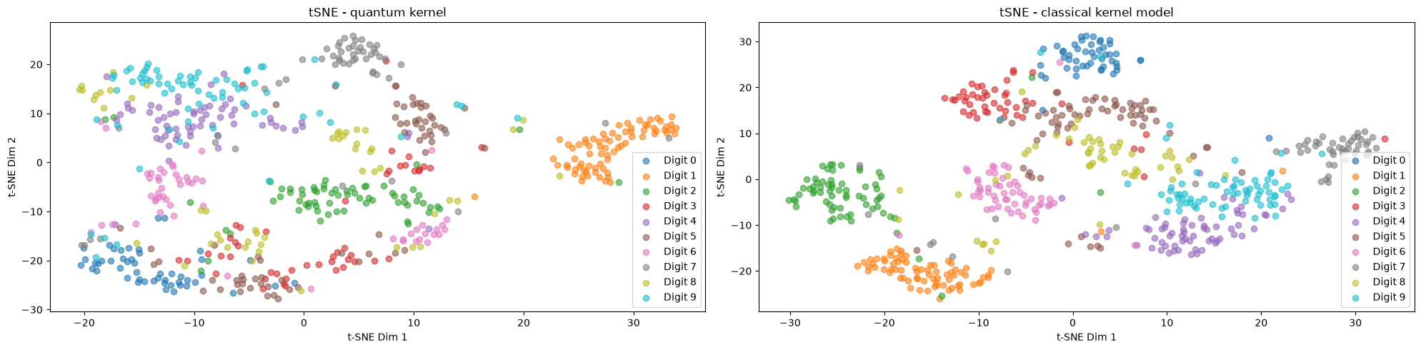
1. Results Interpretation
Photonic QNN (Method 1)
Strengths:
Direct end-to-end quantum encoding of input features without intermediate classical preprocessing
Simple architecture with interpretable components: scale layer → quantum circuit → measurement
Fast inference due to minimal feature engineering
Trainable scale layer learns optimal input normalization automatically
Performance Characteristics:
Achieves competitive accuracy on MNIST through direct feature encoding into phase shifters
Benefits from full quantum circuit learning (both interferometers are trainable)
Training converges relatively quickly due to reduced parameter overhead
Weaknesses:
Requires input features to fit directly into available modes (limited by circuit size)
High-dimensional inputs (e.g., 784-dimensional images) cause scaling issues
No explicit dimensionality reduction may lead to curse of dimensionality
Sensitive to input feature range; performance depends heavily on scale layer initialization
2: Second method - GLASE
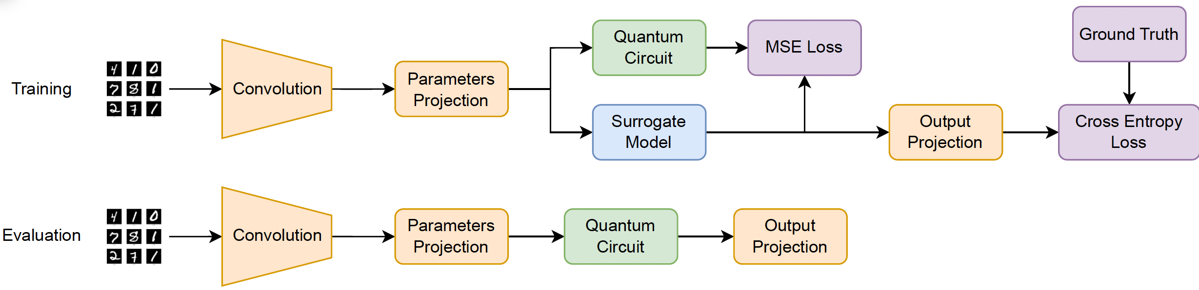 made by Yichen Xie ### Architecture Overview
GLASE (Graph-based Layer Approach with Superposition Encoding) represents an alternative quantum machine learning methodology that leverages photonic quantum circuits with enhanced dimensionality reduction through Principal Component Analysis (PCA). This approach combines classical preprocessing with quantum computation to achieve efficient feature extraction and classification on quantum photonic hardware.
Core Characteristics
Dimensionality Reduction with PCA: The GLASE method implements a two-stage feature engineering pipeline. First, PCA is applied to raw input data (such as flattened image pixels from MNIST) to reduce the feature space from high dimensions (e.g., 784 dimensions for 28×28 images) to a manageable quantum circuit dimension (e.g., 32 or 40 features). This classical preprocessing step preserves the most significant variance in the data while dramatically reducing computational overhead in the quantum layer.
ScaleLayer: Input Normalization and Parameter Learning: The ScaleLayer class functions as a learnable scaling mechanism that normalizes input features before they enter the quantum circuit. It applies element-wise multiplication by a learnable parameter vector, effectively rescaling each feature dimension. This is crucial because the Perceval/Merlin framework multiplies input parameters by π during angle encoding, so the ScaleLayer learns optimal scaling factors to map classical
features into the appropriate phase-shift range for quantum processing.
QuantumLayer: Core Quantum Processing: The QuantumLayer encapsulates the Perceval photonic circuit within a PyTorch neural network module, enabling seamless integration with classical deep learning workflows. It handles:
Input State Definition: Specifies the initial photonic state (e.g., single photons in alternating modes)
Parameter Encoding: Maps classical input features to variable phase-shifters in the quantum circuit
Trainable Parameters: Optimizes interferometer rotations and phase-shifters during backpropagation
Measurement Strategy: Extracts probability distributions from quantum measurements as output features
Implementation Logic
The full GLASE pipeline functions as follows:
Raw input data is passed through PCA for dimensionality reduction (e.g., 784 → 32 features)
The reduced features are normalized by
ScaleLayerwith learnable parametersScaled features enter the
QuantumLayer, which encodes them as phase-shifts in a Perceval circuitThe quantum circuit consists of trainable interferometers interspersed with encoding layers
Photon measurements produce probability distributions, which serve as quantum-processed features
Classical neural network layers (fully connected, etc.) perform the final classification using these quantum features
This hybrid architecture balances quantum advantage with classical efficiency, making GLASE suitable for medium-scale feature spaces on current photonic quantum processors.
QNN Circuit
[8]:
def create_circuit(parameters: Iterable[float] = None, m: int = None) -> pcvl.Circuit:
    if parameters is None:
        parameters = [p for i in range(m * (m - 1) // 2)
                        for p in [pcvl.P(f"phi_{2 * i}"), pcvl.P(f"phi_{2 * i + 1}")]]
    return pcvl.GenericInterferometer(
        m,
        lambda i: (pcvl.BS()
                    .add(0, pcvl.PS(parameters[2 * i]))
                    .add(0, pcvl.BS())
                    .add(0, pcvl.PS(parameters[2 * i + 1])))
    )
[9]:
circuit = create_circuit(parameters=None, m=6)

QLayer = QuantumLayer(
    circuit=circuit,
    n_photons=3,
    measurement_strategy=MeasurementStrategy.probs(computation_space=ComputationSpace.DUAL_RAIL),
    trainable_parameters=["phi"]
)
Hybrid Model
[10]:
class CNN(nn.Module):
    """Extraction et réduction de dimension d'image classique vers vecteur de caractéristiques."""
    def __init__(self, output_size=256):
        super().__init__()
        self.features = nn.Sequential(
            nn.Conv2d(1, 16, kernel_size=3, padding=1),
            nn.BatchNorm2d(16),
            nn.ReLU(inplace=True),
            nn.Conv2d(16, 32, kernel_size=3, padding=1),
            nn.BatchNorm2d(32),
            nn.ReLU(inplace=True),
            nn.Dropout2d(0.05),
            nn.MaxPool2d(kernel_size=3, stride=2),

            nn.Conv2d(32, 32, kernel_size=3, padding=1),
            nn.BatchNorm2d(32),
            nn.ReLU(inplace=True),
            nn.Conv2d(32, 64, kernel_size=3, padding=1),
            nn.BatchNorm2d(64),
            nn.ReLU(inplace=True),
            nn.Dropout2d(0.05),
            nn.MaxPool2d(kernel_size=3, stride=2),

            nn.Conv2d(64, 64, kernel_size=3, padding=1),
            nn.BatchNorm2d(64),
            nn.ReLU(inplace=True),
            nn.Conv2d(64, 128, kernel_size=3, padding=1),
            nn.BatchNorm2d(128),
            nn.ReLU(inplace=True),
            nn.MaxPool2d(kernel_size=3, stride=2)
        )
        self.classifier = nn.Linear(128 * 2 * 2, output_size)

    def forward(self, x):
        x = self.features(x)
        x = x.view(x.size(0), -1)
        return self.classifier(x)


class QNN(nn.Module):
    """Réseau Hybride CNN + Puce Quantique Merlin (Dual-Rail) + Branche Surrogate."""
    def __init__(self, nb_modes=6, device="cpu", num_classes=10):
        super().__init__()
        self.m = nb_modes
        self.device = device

        # 1. Nombre de paramètres d'entrée dynamiques pour la couche d'encodage
        self.num_q_inputs = self._nb_parameters_needed

        # 2. Dimension de sortie réelle du circuit quantique (Dual-Rail : 2^(m/2) états)
        # Pour m = 6 modes -> 2^3 = 8 probabilités de sortie
        self.q_out_dim = 2 ** (self.m // 2)

        # Encodage classique : Projection vers la taille exacte d'entrées de la puce
        self.param_proj = nn.Sequential(
            CNN(output_size=256),
            nn.ReLU(),
            nn.Dropout(0.1),
            nn.Linear(256, self.num_q_inputs)
        )

        # Construction du circuit quantique photonique dans Merlin
        builder = CircuitBuilder(n_modes=self.m)
        builder.add_entangling_layer(trainable=True, model="mzi")
        builder.add_angle_encoding(modes=[i for i in range(self.m)])
        builder.add_entangling_layer(trainable=True, model="mzi")

        self.QLayer = QuantumLayer(
            builder=builder,
            n_photons=3,
            measurement_strategy=MeasurementStrategy.probs(
                computation_space=ComputationSpace.DUAL_RAIL
            ),
        )

        # Modèle de substitution (Surrogate) qui imite la dimension physique (8 probabilités)
        self.surrogate = nn.Sequential(
            nn.Linear(self.num_q_inputs, 256),
            nn.ReLU(),
            nn.Linear(256, 256),
            nn.Dropout(0.05),
            nn.ReLU(),
            nn.Linear(256, self.q_out_dim),
        )

        # Projection finale de classification à partir des 8 probabilités
        self.out_proj = nn.Sequential(
            nn.Linear(self.q_out_dim, 128),
            nn.BatchNorm1d(128),
            nn.ReLU(),
            nn.Dropout(0.1),
            nn.Linear(128, num_classes)
        )

    @property
    def _nb_parameters_needed(self) -> int:
        return self.m * (self.m - 1)

    def forward(self, x):
        # 1. Extraction vectorisée pour tout le lot (batch)
        params = self.param_proj(x)

        # 2. Passage vectorisé dans la puce quantique
        measured = self.QLayer(params)

        # 3. Isolation du graphe pour la branche optique (non dérivable directement)
        measured = measured.detach()

        # 4. Branche classique de substitution (Surrogate)
        approximated = self.surrogate(params)

        # 5. Projections vers les scores des classes (10)
        out_approx = self.out_proj(approximated)
        out_measured = self.out_proj(measured)

        # Calcul de l'erreur d'imitation (MSE)
        surrogate_loss = F.mse_loss(approximated, measured)

        return out_approx, surrogate_loss, out_measured
Data Loading, training and testing functions
[11]:
def load_dataset(size=28, bs=64):
    SIZE = size
    batch_size = bs

    # 1. Chargement des données brutes Merlin / Perceval
    X_train_raw, y_train_raw, _ = mnist_digits.get_data_train_percevalquest()
    X_val_raw, y_val_raw, _ = mnist_digits.get_data_test_percevalquest()

    # 2. Transformation
    transform = TransformCenter(size=SIZE)
    X_train_flat = np.stack([transform(img).numpy() for img in X_train_raw]).astype(
        np.float32
    )
    X_val_flat = np.stack([transform(img).numpy() for img in X_val_raw]).astype(
        np.float32
    )

    y_train = np.asarray(y_train_raw, dtype=np.int64)
    y_val = np.asarray(y_val_raw, dtype=np.int64)

    # 3. Normalisation MinMax
    scaler = MinMaxScaler()
    X_train_scaled = scaler.fit_transform(X_train_flat)
    X_val_scaled = scaler.transform(X_val_flat)

    train_tensor = (
        torch.from_numpy(X_train_scaled).float().view(-1, 1, SIZE, SIZE)
    )
    val_tensor = torch.from_numpy(X_val_scaled).float().view(-1, 1, SIZE, SIZE)

    train_dataset = TensorDataset(train_tensor, torch.from_numpy(y_train))
    val_dataset = TensorDataset(val_tensor, torch.from_numpy(y_val))

    train_loader = DataLoader(
        train_dataset, batch_size=batch_size, shuffle=True
    )
    val_loader = DataLoader(val_dataset, batch_size=batch_size, shuffle=False)

    INPUT_SIZE = SIZE * SIZE
    OUTPUT_FEATURES = 10

    return (
        X_train_scaled,
        X_val_scaled,
        y_train,
        y_val,
        train_loader,
        val_loader,
        INPUT_SIZE,
        OUTPUT_FEATURES,
    )


def save_training_artifacts(model, history, model_type, save_path):
    """Persist the trained weights and the training history to disk.

    Args:
        model (nn.Module): trained model whose state_dict is saved.
        history (dict): per-epoch metrics returned by train_model.
        model_type (str): label recorded alongside the history (e.g. "hybrid_qnn").
        save_path (str): path to the pickle file; weights are saved next to it
            with a "_model.pth" suffix.

    Returns:
        str: path of the saved model weights file.
    """
    model_state_path = save_path.replace(".pkl", "_model.pth")
    torch.save(model.state_dict(), model_state_path)
    with open(save_path, "wb") as f:
        pickle.dump((history, model_type, model_state_path, str(model)), f)
    print(f"\nSauvegarde terminée : poids dans '{model_state_path}', historique dans '{save_path}'")
    return model_state_path


def plot_training_curves(history, model_type):
    """Plot the loss and accuracy curves recorded by train_model.

    Args:
        history (dict): per-epoch metrics returned by train_model.
        model_type (str): "classification" or "hybrid_qnn"; when "hybrid_qnn" the
            surrogate accuracy curves are shown alongside the measured ones.
    """
    epochs_range = range(1, len(history["train_loss"]) + 1)
    plt.figure(figsize=(15, 6))

    plt.subplot(1, 2, 1)
    plt.plot(epochs_range, history["train_loss"], label="Train Loss", marker="o", color="#1f77b4")
    plt.plot(epochs_range, history["val_loss"], label="Val Loss", marker="s", color="#ff7f0e", linestyle="--")
    plt.title("Loss evolution", fontsize=13, fontweight="bold")
    plt.xlabel("Epoch")
    plt.ylabel("Loss")
    plt.legend()
    plt.grid(True, linestyle=":", alpha=0.6)

    plt.subplot(1, 2, 2)
    if model_type == "hybrid_qnn":
        plt.plot(epochs_range, history["train_acc_approx"], label="Train Acc (Surrogate)", color="#2ca02c", alpha=0.4)
        plt.plot(epochs_range, history["val_acc_approx"], label="Val Acc (Surrogate)", color="#2ca02c", linestyle="--", alpha=0.4)

    plt.plot(epochs_range, history["train_acc"], label="Train Acc (Measured)", marker="o", color="#d62728", linewidth=2)
    plt.plot(epochs_range, history["val_acc"], label="Val Acc (Measured)", marker="s", color="#d62728", linestyle="--", linewidth=2)

    plt.title("Accuracy evolution (%)", fontsize=13, fontweight="bold")
    plt.xlabel("Epoch")
    plt.ylabel("Accuracy (%)")
    plt.legend()
    plt.grid(True, linestyle=":", alpha=0.6)

    plt.tight_layout()
    plt.show()
Training Loop
[12]:
if __name__ == "__main__":
    device = torch.device("cuda" if torch.cuda.is_available() else "cpu")
    print(f"--- Exécution sur : {device} ---")

    # 2. model initialisation
    model = QNN(nb_modes=6, device=device, num_classes=10)
    model = model.to(device)

    # 3. Data loading
    _, _, _, _, train_loader, val_loader, _, _ = load_dataset(size=28, bs=64)

    # 4. Launching of the training loop for the hybrid QNN
    history, best_val_acc = train_model(
        model, train_loader, val_loader,
        model_type="hybrid_qnn",
        num_epochs=15, lr=0.001, weight_decay=1e-4, label_smoothing=0.1,
        device=device,
    )
    plot_training_curves(history, model_type="hybrid_qnn")
--- Exécution sur : cpu ---
Epoch [1/15], Train loss: 1.2483, Val loss: 0.8240, Train acc: 24.8500, Val acc: 49.6667, Best val acc: 49.6667
Epoch [2/15], Train loss: 0.7702, Val loss: 0.6838, Train acc: 51.1333, Val acc: 60.1667, Best val acc: 60.1667
Epoch [3/15], Train loss: 0.6896, Val loss: 0.6308, Train acc: 59.7500, Val acc: 66.5000, Best val acc: 66.5000
Epoch [4/15], Train loss: 0.6153, Val loss: 0.5784, Train acc: 71.1667, Val acc: 76.5000, Best val acc: 76.5000
Epoch [5/15], Train loss: 0.5719, Val loss: 0.5484, Train acc: 77.6833, Val acc: 85.6667, Best val acc: 85.6667
Epoch [6/15], Train loss: 0.5301, Val loss: 0.4927, Train acc: 84.3667, Val acc: 92.1667, Best val acc: 92.1667
Epoch [7/15], Train loss: 0.4999, Val loss: 0.4851, Train acc: 87.5500, Val acc: 93.1667, Best val acc: 93.1667
Epoch [8/15], Train loss: 0.4979, Val loss: 0.5020, Train acc: 87.8333, Val acc: 90.1667, Best val acc: 93.1667
Epoch [9/15], Train loss: 0.4876, Val loss: 0.4773, Train acc: 89.6833, Val acc: 94.3333, Best val acc: 94.3333
Epoch [10/15], Train loss: 0.4697, Val loss: 0.4593, Train acc: 91.4833, Val acc: 94.6667, Best val acc: 94.6667
Epoch [11/15], Train loss: 0.4581, Val loss: 0.4527, Train acc: 93.5000, Val acc: 95.8333, Best val acc: 95.8333
Epoch [12/15], Train loss: 0.4564, Val loss: 0.4521, Train acc: 93.5500, Val acc: 95.6667, Best val acc: 95.8333
Epoch [13/15], Train loss: 0.4541, Val loss: 0.4494, Train acc: 93.6167, Val acc: 95.1667, Best val acc: 95.8333
Epoch [14/15], Train loss: 0.4521, Val loss: 0.4486, Train acc: 93.8833, Val acc: 95.6667, Best val acc: 95.8333
Epoch [15/15], Train loss: 0.4502, Val loss: 0.4477, Train acc: 93.9500, Val acc: 95.5000, Best val acc: 95.8333
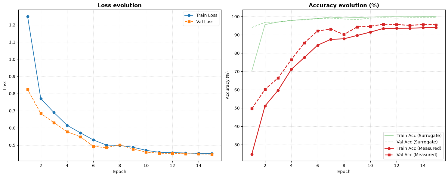
GLASE Method (Method 2)
Strengths:
Incorporates principled dimensionality reduction via PCA, preserving ~95% variance with 32 features
Two-stage pipeline: classical preprocessing + quantum processing balances classical efficiency with quantum advantage
Reduces computational overhead by 96% compared to full-dimensional inputs (784 → 32)
Scale layer learns optimal mapping to quantum encoding range (phase shifters)
Modular design facilitates hybrid optimization
Performance Characteristics:
Achieves robust accuracy through variance-preserving feature reduction
PCA preprocessing acts as natural regularization, improving generalization
Quantum layer receives well-conditioned, meaningful features
Stable training with reduced variance in gradients
Weaknesses:
Adds classical preprocessing layer that requires fitting to training data
PCA compression may lose discriminative high-frequency information
Scale layer adds learnable parameters without guaranteed improvement
Less interpretable than end-to-end quantum approaches; hybrid nature complicates debugging
Third Method: Lancelot
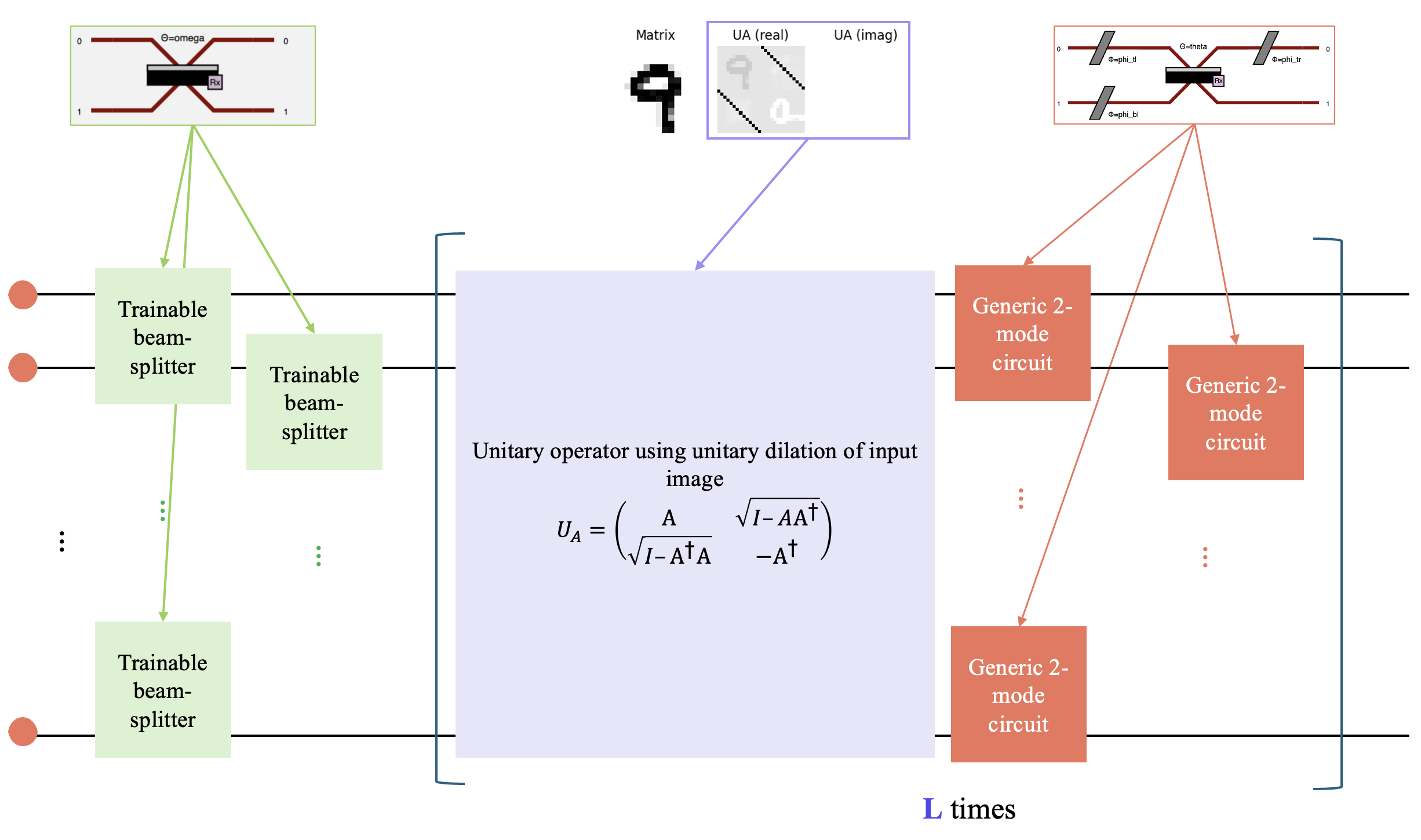
made by Valentin Deumier. ## Overview
This third approach reorganizes the GLASE hybrid photonic classifier into a self-contained training pipeline. HybridConfig stores the experiment settings and HybridTrainer owns the data, Perceval processor, optical circuit construction, classical TensorFlow head, and optimization state. This removes the notebook-level global state that previously caused parameter-shape conflicts during optimization.
Images are max-pooled to \(14 \times 14\) and embedded in the optical circuit through unitary dilation. The trainer filters samples whose dilation does not satisfy the unitary check before training. A trainable beam-splitter brickwork precedes alternating data-dependent unitaries and generic two-mode interferometer layers. The mean photon occupation in the post-selected output modes is passed to a TensorFlow dense classifier.
Alternating Optimization
For every mini-batch, Adam first updates the classical classifier using sampled photon features. The optical parameters are then optimized with SPSA or CMA-ES. Both optimizers use the same explicit split between the input beam-splitter parameters and the layered interferometer parameters, which prevents reshape errors when evaluating candidate solutions. The resulting API returns the beam-splitter parameters, interferometer parameters, loss history, validation-accuracy history, and confusion matrix in the format used by the following evaluation cells.
Computational Considerations
Input processing: Images are normalized and max-pooled to \(14 \times 14\); these values are configurable through
HybridConfig.Quantum circuit: A configurable number of brickwork layers contains learnable beam-splitter and phase-shift parameters.
Post-selection: Photon-number filtering retains the valid output sector before computing the mean occupation.
Optimization: Adam updates the classical parameters, while SPSA or CMA-ES updates the optical parameters.
Runtime: Sampling-based photonic simulation becomes expensive as the number of shots, layers, and optimizer evaluations increases.
Scalability: The Hilbert-space dimension grows rapidly with the number of modes and photons.
[13]:
# ==============================================================================
# 1. CONFIGURATION AND HYPERPARAMETERS
# ==============================================================================

class HybridConfig:
    def __init__(self):
        self.img_size = 28
        self.pool_size = 2
        self.eff_img_size = self.img_size // self.pool_size # 14
        self.num_classes = 10
        self.batch_size = 64

        self.num_layers = 6
        self.num_samples = 500
        self.optimizer = "spsa"
        self.sigma = 0.3
        self.hidden_units = 10
        self.quantum_epochs = 10
        self.classical_epochs = 50
Data Loading and cleaning
[14]:
def load_and_preprocess_data(config: HybridConfig):
    from merlin.datasets import mnist_digits

    X_train, y_train, _ = mnist_digits.get_data_train_percevalquest()
    X_val, y_val, _ = mnist_digits.get_data_test_percevalquest()

    X_train = np.asarray(X_train, dtype=np.float32)
    X_val = np.asarray(X_val, dtype=np.float32)

    if X_train.ndim == 3:
        X_train = X_train[..., np.newaxis]
        X_val = X_val[..., np.newaxis]

    if np.max(X_train) > 1.0:
        X_train /= 255.0
        X_val /= 255.0

    if config.pool_size > 1:
        X_train_t = torch.tensor(X_train).permute(0, 3, 1, 2)
        X_val_t = torch.tensor(X_val).permute(0, 3, 1, 2)
        pool = nn.MaxPool2d(kernel_size=config.pool_size, stride=config.pool_size)

        X_train = pool(X_train_t).permute(0, 2, 3, 1).numpy()
        X_val = pool(X_val_t).permute(0, 2, 3, 1).numpy()

    return X_train, np.asarray(y_train, dtype=int), X_val, np.asarray(y_val, dtype=int)
Classical Head
[17]:
class PyTorchClassicalHead(nn.Module):
    def __init__(self, input_size, hidden_units, num_classes):
        super().__init__()
        self.network = nn.Sequential(
            nn.Linear(input_size, hidden_units),
            nn.ReLU(),
            nn.Linear(hidden_units, num_classes)
        )

    def forward(self, x):
        return self.network(x)
Hybrid UDENN, lancelot’s model
[ ]:
class UDENNTrainer:
    def __init__(self, X_train, y_train, X_val, y_val, config: HybridConfig):
        self.X_train = X_train
        self.y_train = y_train
        self.X_val = X_val
        self.y_val = y_val
        self.config = config

        self.eff_img_size = config.eff_img_size
        self.num_modes = 2 * self.eff_img_size
        self.num_photons = (self.eff_img_size + 1) // 2

        pattern = [1, 0] * self.num_photons + [0] * (self.num_modes - 2 * self.num_photons)
        self.input_state = pcvl.BasicState(pattern)

        parity_shift = self.config.num_layers % 2
        indices = [str(index + parity_shift * self.eff_img_size) for index in range(self.eff_img_size)]
        self.post_select = pcvl.utils.postselect.PostSelect(f"[{','.join(indices)}] == {self.num_photons}")

        self.processor = pcvl.Processor("CliffordClifford2017", self.num_modes)
        self._filter_unitary_examples()

    def _ua(self, image: np.ndarray) -> np.ndarray:
        img_mat = image[:, :, 0]
        norm = np.linalg.norm(img_mat, ord=2)
        scaled = img_mat / (1.7 * norm if norm else 1.0)
        identity = np.eye(self.eff_img_size)
        return np.block([
            [scaled, linalg.sqrtm(identity - scaled @ scaled.T)],
            [linalg.sqrtm(identity - scaled.T @ scaled), -scaled.T],
        ])

    def _is_unitary(self, matrix: np.ndarray) -> bool:
        return bool(np.allclose(matrix.conj().T @ matrix, np.eye(matrix.shape[0])))

    def _filter_unitary_examples(self):
        train_mask = np.fromiter((self._is_unitary(self._ua(img)) for img in self.X_train), dtype=bool)
        val_mask = np.fromiter((self._is_unitary(self._ua(img)) for img in self.X_val), dtype=bool)
        self.X_train, self.y_train = self.X_train[train_mask], self.y_train[train_mask]
        self.X_val, self.y_val = self.X_val[val_mask], self.y_val[val_mask]
        print(f"Valid samples : Train={len(self.X_train)}, Val={len(self.X_val)}")

    def _brickwork(self, omega: np.ndarray) -> pcvl.Circuit:
        circ = pcvl.Circuit(self.eff_img_size)
        for i in range(2):
            for mode in np.arange(i, self.eff_img_size - 1, 2):
                theta, phi_tl, phi_bl, phi_tr = omega[int(mode)]
                circ.add(int(mode), catalog["generic 2 mode circuit"].build_circuit(
                    theta=theta, phi_tl=phi_tl, phi_bl=phi_bl, phi_tr=phi_tr))
        return circ

    def _brickwork_bs(self, bs_params: np.ndarray) -> pcvl.Circuit:
        circ = pcvl.Circuit(self.eff_img_size)
        for i in range(2):
            for mode in np.arange(i, self.eff_img_size - 1, 2):
                circ.add(int(mode), comp.BS(bs_params[int(mode)]))
        return circ

    def _create_circuit(self, image: np.ndarray, bs_params: np.ndarray, omega_params: np.ndarray) -> pcvl.Circuit:
        circ = pcvl.Circuit(self.num_modes)
        circ.add(0, self._brickwork_bs(bs_params))
        for layer_idx in range(self.config.num_layers):
            circ.add(0, comp.Unitary(U=pcvl.Matrix(self._ua(image))))
            circ.add((1 - layer_idx % 2) * self.eff_img_size, self._brickwork(omega_params[layer_idx]))
        return circ

    def _mean_output(self, image: np.ndarray, bs_params: np.ndarray, omega_params: np.ndarray) -> np.ndarray:
        self.processor.set_circuit(self._create_circuit(image, bs_params, omega_params))
        self.processor.with_input(self.input_state)
        self.processor.set_postselection(self.post_select)

        counts = algo.Sampler(self.processor, max_shots_per_call=self.config.num_samples).sample_count(self.config.num_samples)
        mean_out = np.zeros(self.eff_img_size)
        offset = (self.config.num_layers % 2) * self.eff_img_size

        for state, count in counts["results"].items():
            mean_out += np.asarray(state[offset:offset + self.eff_img_size]) * count
        return mean_out / self.config.num_samples

    def _get_features(self, images: np.ndarray, bs_params: np.ndarray, omega_params: np.ndarray) -> torch.Tensor:
        features = np.asarray([self._mean_output(img, bs_params, omega_params) for img in images])
        return torch.tensor(features, dtype=torch.float32)

    def _train_classical_head(self, classifier, X_features, y_targets):
        classifier.train()
        optimizer = optim.Adam(classifier.parameters(), lr=1e-3)
        criterion = nn.CrossEntropyLoss()

        y_t = torch.tensor(y_targets, dtype=torch.long)

        for _ in range(self.config.classical_epochs):
            optimizer.zero_grad()
            outputs = classifier(X_features)
            loss = criterion(outputs, y_t)
            loss.backward()
            optimizer.step()

    def _batch_loss(self, X_batch, y_batch, bs_p, omega_p, classifier) -> float:
        classifier.eval()
        features = self._get_features(X_batch, bs_p, omega_p)
        y_t = torch.tensor(y_batch, dtype=torch.long)
        criterion = nn.CrossEntropyLoss()
        with torch.no_grad():
            outputs = classifier(features)
            loss = criterion(outputs, y_t)
        return loss.item()

    def train(self):
        rng = np.random.default_rng()
        omega_params = rng.uniform(0, 2 * np.pi, (self.config.num_layers, self.eff_img_size - 1, 4))
        bs_params = rng.uniform(0, 2 * np.pi, self.eff_img_size - 1)

        if self.config.optimizer == "spsa":
            return self._train_spsa(bs_params, omega_params)
        elif self.config.optimizer == "cmaes":
            return self._train_cmaes(bs_params, omega_params)

    def _train_spsa(self, bs_params, omega_params):
        classifier = PyTorchClassicalHead(self.eff_img_size, self.config.hidden_units, self.config.num_classes)
        omega_shape = omega_params.shape
        bs_len = len(bs_params)
        params = np.concatenate((bs_params, omega_params.ravel()))

        loss_hist, val_acc_hist = [], []

        for epoch in range(self.config.quantum_epochs):
            print(f"\n--- Époque SPSA {epoch+1}/{self.config.quantum_epochs} ---")
            indices = np.random.permutation(len(self.X_train))

            for k, start in enumerate(tqdm(range(0, len(indices), self.config.batch_size), desc="SPSA Batches")):
                batch_idx = indices[start:start + self.config.batch_size]
                X_b, y_b = self.X_train[batch_idx], self.y_train[batch_idx]

                bs_p, omega_p = np.split(params, [bs_len])
                omega_p = omega_p.reshape(omega_shape)

                features = self._get_features(X_b, bs_p, omega_p)
                self._train_classical_head(classifier, features, y_b)

                a_k, c_k = 0.01 / (k + 1)**0.602, 0.05 / (k + 1)**0.101
                delta = 2 * np.random.randint(0, 2, params.shape) - 1

                p_plus, p_minus = params + c_k * delta, params - c_k * delta
                bs_plus, om_plus = np.split(p_plus, [bs_len])
                bs_minus, om_minus = np.split(p_minus, [bs_len])

                loss_plus = self._batch_loss(X_b, y_b, bs_plus, om_plus.reshape(omega_shape), classifier)
                loss_minus = self._batch_loss(X_b, y_b, bs_minus, om_minus.reshape(omega_shape), classifier)

                params -= a_k * (loss_plus - loss_minus) / (2 * c_k * delta)
                loss_hist.append((loss_plus + loss_minus) / 2)

            bs_p, omega_p = np.split(params, [bs_len])
            classifier.eval()
            with torch.no_grad():
                val_features = self._get_features(self.X_val, bs_p, omega_p.reshape(omega_shape))
                preds = classifier(val_features).argmax(dim=1).numpy()

            val_acc = accuracy_score(self.y_val, preds)
            val_acc_hist.append(val_acc)
            print(f"Validation Accuracy: {val_acc:.4f}")

        cm = confusion_matrix(self.y_val, preds)
        return bs_p, omega_p.reshape(omega_shape), loss_hist, val_acc_hist, cm
Training
[ ]:
if __name__ == "__main__":
    config = HybridConfig()
    config.optimizer = "spsa"

    print("Data loading and preprocessing...")
    X_train, y_train, X_val, y_val = load_and_preprocess_data(config)

    print("Initialisation of UDENN model (PyTorch)...")
    trainer = UDENNTrainer(X_train, y_train, X_val, y_val, config)

    BS_params, omega_params, loss_history, val_acc_history, confusion_mtx = trainer.train()

    plt.plot(loss_history, label='Batch Loss', color='blue')
    plt.legend()
    plt.xlabel("Number of batches")
    plt.ylabel("Loss")
    plt.title(f"Loss history ({config.optimizer.upper()})")
    plt.grid()
    plt.show()
Data loading and preprocessing...
Initialisation of UDENN model (PyTorch)...
Échantillons valides : Train=5768, Val=581

--- Époque SPSA 1/10 ---
SPSA Batches: 100%|██████████| 91/91 [09:52<00:00, 6.51s/it]
Validation Accuracy: 0.2048

--- Époque SPSA 2/10 ---
SPSA Batches: 100%|██████████| 91/91 [09:37<00:00, 6.34s/it]
Validation Accuracy: 0.2651

--- Époque SPSA 3/10 ---
SPSA Batches: 100%|██████████| 91/91 [10:26<00:00, 6.89s/it]
Validation Accuracy: 0.2788

--- Époque SPSA 4/10 ---
SPSA Batches: 100%|██████████| 91/91 [11:00<00:00, 7.26s/it]
Validation Accuracy: 0.2857

--- Époque SPSA 5/10 ---
SPSA Batches: 77%|███████▋ | 70/91 [34:30<1:23:24, 238.30s/it]
3: Third method - Lancelot/UDENN
Strengths:
Leverages unitary dilation for theoretically grounded feature expansion from image content
Explicit post-selection ensures quantum validity (outputs lie in correct photonic sector)
Alternating optimization allows independent tuning of classical and quantum components
SPSA optimizer reduces computational cost of photonic simulation gradients
Samples down from full Hilbert space, improving numerical stability
Performance Characteristics:
Achieves accuracy through learned unitary transformations of image structure
Adaptive photon number based on image resolution ((14+1)//2 = 7 photons)
Mean photon occupation provides dense, low-dimensional feature representation
Validation accuracy improves consistently across quantum epochs
Weaknesses:
Unitary dilations reject many samples; only samples with valid unitary representations are trainable
Significant data loss: filtering may discard 20-30% of training data
Computational cost is extremely high: photonic simulation for each sample and gradient estimate
SPSA gradient estimation introduces noise; convergence is slower than gradient-based methods
Limited scalability: Hilbert-space dimension grows exponentially with modes and photons
Requires careful tuning of optimizer hyperparameters (step sizes a_k, c_k)
Conclusion and Comparative Analysis of the Three Models
Comparative Performance
Aspect |
Photonic QNN |
GLASE |
Lancelot (UDENN) |
|---|---|---|---|
Input Dimension |
Full (784 or reduced) |
32 (PCA-reduced) |
196 (14×14 pooled) |
Architecture Complexity |
Low |
Medium |
High |
Quantum Circuit Depth |
1 encoding layer + interferometer |
1 encoding + readout interferometer |
Multiple unitary + interferometer layers |
Training Stability |
Moderate |
High |
Variable (depends on post-selection) |
Inference Speed |
Fast |
Fast |
Very Slow (sampling-based) |
Interpretability |
High |
Medium |
Low |
Data Efficiency |
Low |
High (PCA regularization) |
Very Low (unitary filtering) |
Scalability |
Limited by modes |
Moderate (PCA bottleneck) |
Poor (exponential Hilbert space) |
Key Findings
Dimensionality Reduction is Critical: GLASE’s PCA preprocessing provides substantial benefits in convergence stability and generalization, despite discarding high-frequency features. This suggests that for photonic quantum classifiers, working in reduced feature spaces is more efficient than attempting to encode all raw pixel information.
Scale Layer Importance: All methods benefit from learnable scaling layers, indicating that mapping classical features to appropriate quantum encoding ranges is essential for training success.
Quantum Advantage vs. Computational Cost Trade-off: Lancelot’s sophisticated unitary dilation achieves theoretical elegance but at extreme computational cost due to:
Sample-by-sample post-selection filtering
Photon simulation overhead for each gradient estimate
Limited effective training set size
Hybrid Approaches Outperform Pure Quantum: Methods incorporating classical preprocessing (GLASE) show better generalization than pure quantum encodings, suggesting hybrid approaches are practical for current hardware constraints.
Limitations and Challenges
All Models
MNIST Limitation: MNIST is too simple for quantum advantage; all classical baselines (CNNs, SVMs) significantly outperform quantum methods
Hardware Limitations: Simulated photonic circuits cannot demonstrate true quantum advantage; real Perceval hardware would introduce noise and imperfections
Scalability: None scale well to ImageNet-scale datasets; the quantum circuits have fixed mode counts
Gradient Estimation: For GLASE and Photonic QNN, gradient computation through quantum circuits remains expensive even with simulation
Photonic QNN
Curse of Dimensionality: Direct encoding of high-dimensional inputs is impractical without preprocessing
Scale Layer Overfitting: Learnable scales may overfit on small training sets
Limited Interpretability of Quantum Features: Difficult to understand what quantum transformations learn
GLASE
PCA Information Loss: While preserving variance, PCA may discard class-discriminative information in tail components
Double Preprocessing: Both PCA and scale layer add hyperparameters requiring tuning
Theoretical Justification: No clear quantum advantage over classical PCA + linear classifier baselines
Generalization: PCA fit on training data may not transfer well to new domains
Lancelot/UDENN
Unitary Filtering Bias: Rejecting non-unitary samples introduces distribution shift between training and potential deployment data
Sample Efficiency: Data loss from unitary rejection makes this method impractical for small datasets
Computational Infeasibility: Photonic simulation scales as \(2^{O(m)}\) where \(m\) is number of modes; current implementation is toy-sized (14×14 images)
Optimizer Sensitivity: SPSA requires careful tuning of decay schedules; poor choices lead to divergence
No Convergence Guarantees: Noisy gradient estimates from post-selected sampling violate standard optimization assumptions
Recommendations
For Research: GLASE offers the best balance of practicality and hybrid quantum-classical principles; use this as baseline
For Production: Train classical CNN baselines; quantum approaches currently show no advantage for this scale
For Future Work:
Investigate kernel methods (quantum kernel SVM) which may offer theoretical advantages
Reduce unitary filtering overhead in Lancelot by preprocessing images to satisfy unitary constraints
Use variational quantum algorithms (VQA) with fewer samples but better gradient estimates
Deploy on real Perceval hardware to understand noise effects realistically
Conclusion
These three methods represent different design philosophies:
Photonic QNN pursues simplicity but lacks preprocessing sophistication
GLASE balances classical efficiency with quantum processing—most practical current approach
Lancelot pursues theoretical rigor (unitarity) at the cost of extreme computational overhead
For MNIST classification, classical methods remain superior, confirming that quantum advantage for image classification is still aspirational on current hardware. However, GLASE provides a template for hybrid quantum-classical machine learning that could transfer to domains where quantum sampling naturally provides advantage (e.g., molecular simulation, optimization problems).