Basic Concepts
This guide introduces the fundamental concepts behind Merlin’s approach to quantum neural networks.
Merlin centres on three high-level tools you will see throughout the quickstart:
Photonic simulation with fast classical solvers so you can prototype locally before targeting hardware.
CircuitBuilder for declaratively authoring interferometers, encoding steps, and trainable components.
QuantumLayer for dropping your circuit into any PyTorch model with automatic differentiation support.
Conceptual Overview
Merlin bridges the gap between physical quantum circuits and high-level machine learning interfaces through a layered architecture. From lowest to highest level:
Physical Quantum Circuits: The actual photonic hardware (or fast simulation thereof)
Photonic Backend: Mathematical models of quantum circuits with configurable components
CircuitBuilder (
CircuitBuilder): Declarative interface for assembling photonic circuitsEncoding: Strategies for mapping classical features to quantum parameters
Measurement Strategy: Strategies for converting quantum outputs to classical outputs
QuantumLayer: High-level PyTorch interface that combines all these concepts
Let’s explore each level in detail.
1. Physical Foundation: Photonic Circuits
At the foundation, Merlin uses photonic quantum computing, where information is encoded in photons (particles of light) traveling through optical circuits. These circuits consist of:
Modes: Independent optical pathways (like waveguides) that can carry photons
Photons: Quantum information carriers; more photons enable more complex quantum interference
Optical Components: Beam splitters, phase shifters, and interferometers that manipulate photon paths
On the image above, you can see a 12-mode interferometer with 6 photons entering. The photons interfere as they pass through the optical components, creating complex quantum states. We measure the output distribution of photons across the modes to extract information. Here, we could write
# A simple photonic system
n_modes = 12        # 4 optical pathways
n_photons = 6     # 2 photons for quantum interference
input_state = pcvl.BasicState("|1, 0, 1, 0, 1, 0, 1, 0, 1, 0, 1, 0>")  # Alternating photon pattern
For a deeper understanding of photonic quantum computing fundamentals, see Quantum Architectures.
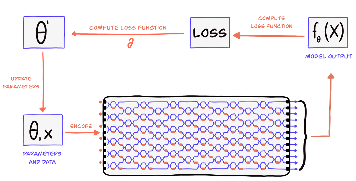
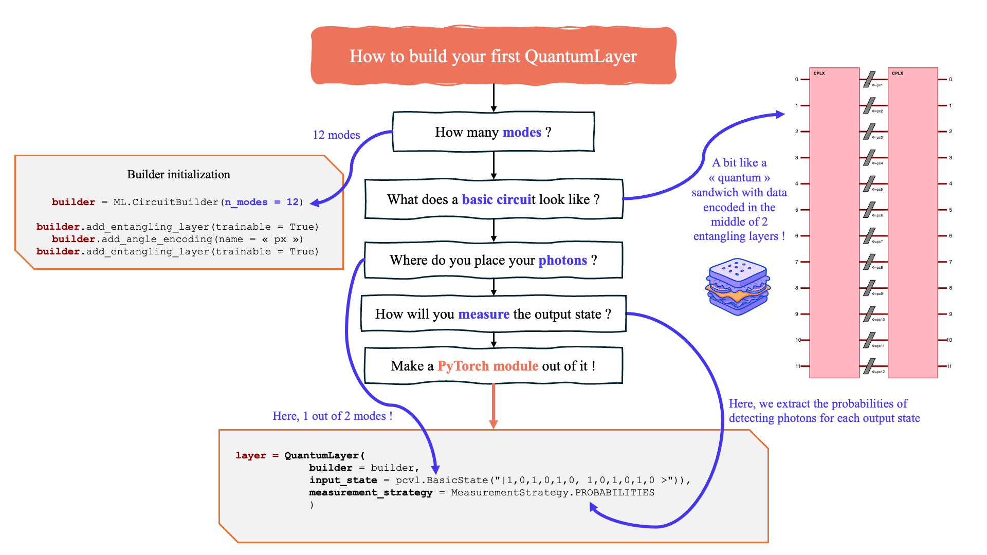
First, we present the overview of the building of a QuantumLayer, brick by brick using the CircuitBuilder.
Overview of the Merlin hybrid workflow.
2. Backend : Mathematical Models
To run this layer, the Backend provides mathematical representations of quantum circuits, handling the complex quantum mechanics while exposing a clean interface for machine learning.
Key responsibilities:
State Evolution: Computing how quantum states change through the circuit (see SLOS: Strong Linear Optical Simulator)
Simulation Modes: Switching between sampling and deterministic simulation for rapid prototyping
Parameter Management: Tracking which components are configurable vs. fixed
Measurement Simulation: Converting quantum states to probability distributions
Merlin comes with high-performance classical simulators (SLOS and Clifford-based modes) so you can prototype and train without immediate access to hardware. Switching to hardware later only requires changing the backend configuration.
3. Encoding: Classical-to-Quantum Mapping
Encoding defines how classical input features are mapped to quantum circuit parameters. This is crucial because quantum circuits operate on phases and amplitudes, not raw feature values.
Key Steps:
Normalization: Ensure inputs are in \([0,1]\) range
Scaling: Apply scaling for quantum parameter ranges
Circuit Mapping: Distribute to quantum parameters based on the configured circuit
Angle Encoding
Angle encoding rotates programmable elements of the circuit by an angle proportional to each classical feature.
import merlin as ML
import numpy as np

builder = ML.CircuitBuilder(n_modes=4)
builder.add_angle_encoding(scale=np.pi)    # Rotations proportional to input features
Angle encoding keeps circuit depth compact while still giving continuous control over the interferometer. Keep signals normalized (or pass them through a bounded activation such as torch.tanh) so the mapped rotation angles remain in a sensible range.
Amplitude Encoding
Amplitude encoding maps classical data directly into the amplitudes of a quantum state. Rather than turning features into phase-shifter angles, you represent your data as the quantum state itself and the circuit acts as a learned unitary transformation on it. The feature vector length must match the Fock basis size \(d = \binom{n\_modes + n\_photons - 1}{n\_photons}\).
Wrap your real-valued data with
StateVector.from_tensor()
and pass the result to forward() — the layer detects the type and activates
amplitude encoding automatically:
import torch
from merlin.core.state_vector import StateVector

features = torch.randn(8, 10)          # batch of 8, d = 10 (4 modes, 2 photons)
sv = StateVector.from_tensor(features, n_modes=4, n_photons=2)
output = layer(sv)                     # shape: (8, output_size)
For a detailed comparison of angle vs. amplitude encoding and complete runnable examples, see Angle Encoding and Amplitude Encoding.
Initial State Patterns
The initial distribution of photons affects quantum behavior:
# Example state patterns
ML.StatePattern.PERIODIC     # occupations: [1, 0, 1, 0] (alternating photons)
ML.StatePattern.SPACED       # occupations: [1, 0, 0, 1] (evenly spaced)
ML.StatePattern.SEQUENTIAL   # occupations: [1, 1, 0, 0] (consecutive)
You can build a concrete input state as a Perceval BasicState with
ML.generate_state(n_modes, n_photons, pattern).
Different patterns create different types of quantum interference and correlations.
For detailed encoding strategies and optimization techniques, see Angle Encoding and Amplitude Encoding.
4. Measurement Strategy: Quantum-to-Classical Conversion
Measurement Strategy converts quantum measurement results (probability distributions or amplitudes) into classical outputs.
Quantum circuits produce probability distributions or amplitudes (in simulation) over possible photon configurations. Measurement strategy determines which formatting to use.
# Common measurement strategies
ML.MeasurementStrategy.probs()              # Default: full probability distribution
ML.MeasurementStrategy.mode_expectations()  # Per-mode photon statistics
ML.MeasurementStrategy.amplitudes()         # Complex amplitudes (simulation only)
To reduce the dimensionality of the Fock distribution after measurement, compose your layer with a grouping
LexGrouping or ModGrouping.
Key Concept: Measurement strategy bridges the gap between quantum measurements and classical outputs. The choice affects both the interpretability and expressivity of your quantum layer.
For detailed comparisons and selection guidelines, see Measurement Strategy Guide and Grouping Guide.
Grouping strategies
Two simple, built-in grouping strategies are provided to reduce the high-dimensional Fock outputs to a smaller set of classical features:
LexGrouping: assigns consecutive output indices to the same bucket (lexicographicordering). This preserves locality in the Fock index ordering and is a good default when nearby basis states are expected to encode related features.
ModGrouping: maps output indices to buckets using a modulo operation, effectivelyinterleaving states across groups. This is useful when you want to mix information from distant basis states or avoid clustering correlated states into the same bucket.
Example:
# Collapse the Fock output into 3 features by grouping consecutive indices
grouped_layer = ML.LexGrouping(quantum_layer.output_size, 3)

# Alternatively, interleave states into 3 groups
interleaved = ML.ModGrouping(quantum_layer.output_size, 3)
5. High-Level Interface: QuantumLayer
The QuantumLayer combines all these concepts into a PyTorch-compatible interface that plays nicely with standard deep learning tooling. Build a circuit with the builder interface, then pass it to the layer alongside the parameters you want Merlin to manage:
import merlin as ML
import numpy as np
from merlin.core.state_vector import StateVector

builder = ML.CircuitBuilder(n_modes=6)
builder.add_angle_encoding(name="px", modes=[0, 1, 2, 3], scale=np.pi)
builder.add_entangling_layer(trainable=True)

quantum_layer = ML.QuantumLayer(
    input_size=4,                                   # Classical feature dimension
    builder=builder,                                # CircuitBuilder instance
    n_photons=2,                                    # Number of photons in the register
    input_state=StateVector.from_basic_state([1, 0, 0, 1, 0, 0]),  # Initial photon pattern
    measurement_strategy=ML.MeasurementStrategy.probs(ML.ComputationSpace.FOCK),
    return_object=False                             # Choose whether or not to return a typed object after a forward call
                                                    # depending on the measurement strategy. Default is False.
)

# Optional: down-sample the Fock distribution to 3 features using a Linear Layer
mapped_layer = nn.Sequential(
    quantum_layer,
    nn.Linear(quantum_layer.output_size, 3),
)
Key parameters to tune when instantiating QuantumLayer:
builderorcircuit: define the photonic circuit you want to simulate.n_photonsandinput_state: set the quantum resources entering the interferometer. The preferred type forinput_stateisStateVector, which bundles amplitudes with Fock metadata and supports superposition inputs that plain lists cannot express. Lists,pcvl.BasicState, andpcvl.StateVectorare also accepted.input_parameters: prefixes generated byadd_angle_encoding(). Derived automatically when abuilderis provided; only needed with a barecircuit.measurement_strategy: pick the classical readout and computation space via the factory methods.probs(),.mode_expectations(),.amplitudes(), or.partial(). TheComputationSpaceis passed as a parameter to the factory (e.g.MeasurementStrategy.probs(ComputationSpace.FOCK)).return_object: Choose to return a typed object as the forward output depending on themeasurement_strategy. The default value is False. Take a look at merlin.algorithms.layer module for more details about the return types.
Encoding mode is inferred from the input type
The layer decides between angle and amplitude encoding based on what you pass to
forward():
Real
torch.Tensor→ angle encoding (features mapped to phase shifters).StateVector→ amplitude encoding (usefrom_tensor()for classical data).Complex
torch.Tensor→ amplitude encoding (tensor variant).
No special constructor flags are needed — just pass the right type.
Typed outputs with return_object=True
By default, the output of the QuantumLayer’s forward function is a torch.Tensor. However if the parameter return_object is set to True in the initialization
(it is False by default), the layer returns typed Merlin objects instead of bare tensors, carrying metadata such as mode count, photon number, and computation space:
.probs()→ProbabilityDistribution, an object that regroups all of the possible outcomes and their probabilities.For more details, merlin.core.probability_distribution.
.amplitudes()→StateVector, an object that regroups all of the possible state_vectors at the end of the circuit and their basis state decomposition.For more details, merlin.core.state_vector.
.mode_expectations()→torch.Tensor
Even when return_object=False,
- .partial() → PartialMeasurement, an object that regroups all of the measurement results and possible output StateVectors.
For more details, merlin.core.partial_measurement.
Putting It All Together
Here’s how all these concepts work together in practice:
import torch
import torch.nn as nn
import merlin as ML
import numpy as np
from merlin.core.state_vector import StateVector

class HybridModel(nn.Module):
    def __init__(self):
        super().__init__()

        # Classical preprocessing
        self.classical_input = nn.Linear(8, 4, bias=False)

        # Quantum processing layer
        builder = ML.CircuitBuilder(n_modes=6)
        builder.add_angle_encoding(name="px", modes=[0, 1, 2, 3], scale=np.pi)
        builder.add_entangling_layer(trainable=True)
        builder.add_superpositions(trainable=True)

        quantum_core = ML.QuantumLayer(
            input_size=4,
            builder=builder,
            n_photons=2,
            input_state=StateVector.from_basic_state([1, 0, 0, 1, 0, 0]),
            measurement_strategy=ML.MeasurementStrategy.probs(ML.ComputationSpace.FOCK),
        )
        self.quantum = nn.Sequential(
            quantum_core,
            # Lexicographic grouping: collapse the high-dimensional Fock output into `6` buckets
            # by assigning consecutive output indices to the same group. This preserves local
            # structure in the Fock ordering and is useful when nearby basis states encode
            # similar features.
            ML.LexGrouping(quantum_core.output_size, 6),
        )

        # Classical output
        self.classifier = nn.Linear(6, 3)

    def forward(self, x):
        x = self.classical_input(x)
        x = torch.sigmoid(x)           # Normalize for quantum encoding
        x = self.quantum(x)            # Quantum transformation
        return self.classifier(x)

# The quantum stack automatically handles:
# - Photonic backend simulation
# - Classical-to-quantum encoding
# - Quantum computation
# - Quantum-to-classical measurement (plus optional grouping)
Design Guidelines
When choosing configurations, consider these general principles:
Start Simple: Begin with a small CircuitBuilder (4–6 modes), default .probs() measurement, and a lightweight classical head.
Match Complexity to Problem:
Simple problems → few modes, shallow entangling layers
Complex problems → more modes, combine entangling layers with superpositions
Computational Constraints:
Limited resources → fewer photons, prefer
ComputationSpace.UNBUNCHEDwhen your circuit avoids photon bunchingMore resources available → increase photon count or depth for richer expressivity
Experiment Systematically: The quantum advantage often comes from the right combination of circuit design, encoding, measurement strategy, and optional grouping for your specific problem.
For detailed optimization strategies and advanced configurations, see the User Guide section.
Next Steps
Now that you understand the conceptual hierarchy:
Start Simple: Prototype with
CircuitBuilderdefaults and the built-in simulatorExperiment: Try different CircuitBuilder layouts, measurement strategies, and grouping modules for your use case
Optimize: Tune circuit size and encoding strategies based on performance
Advanced Usage: Explore custom circuit definitions when needed
For practical implementation, continue to Your First Quantum Layer to see these concepts in action.